DIRECT COMPUTATION OF DEPTH FROM SHADING FOR
PERSPECTIVE PROJECTION
Kousuke Wakabayashi, Norio Tagawa and Kan Okubo
Graduate School of System Design, Tokyo Metropolitan University, Hino-shi, Tokyo, Japan
Keywords:
Depth Recovery, Direct Computation, Shape from Shading, Perspective Projection.
Abstract:
We present a method for recovering shape from shading in which the surface depth is directly computed.
The already proposed method solving the same problem assumes that images are captured under the parallel
projection, and hence, it can be correctly used only for the relative thin objects compared with the distance from
the camera. If this method is formally extended for the perspective projection completely, the complicated
calculations for differential are required. This gives rise to unstable recovery. In this study, we examine an
extension of this method so as to treat the perspective projection approximately. In order to keep the simplicity
of the original method, we propose the simple approximation of the derivative of the surface with respect to
the image coordinate.
1 INTRODUCTION
Various algorithms for shape from shading have
been enthusiastically studied, but most of them com-
pute the surface orientation rather than surface depth
(Brooks and Horn, 1985), (Szeliski, 1991), (Zhang
et al., 1999). Computing surface orientation gives
rise to two fundamental difficulties. First, the recov-
ering problem is under-constrained, i.e. for the each
point in an image, there is one observation but two un-
known. To solve this problem, additional constraints,
such as smoothness of the orientations, are required
to obtain a unique solution. Secondly, arbitrary two
functions p(x,y) and q(x,y) on an image will not gen-
erally correspond to the orientations of some continu-
ous and differential surface.
Horn (Horn, 1990) developed a method which
considered solving for three functions simultane-
ously: a surface function Z(x, y) was recovered in ad-
dition to p(x, y) and q(x, y), which should represent
the surface orientation. In this paper, we use the cap-
ital letter (X,Y,Z) for a three-dimensional point and
the small case letter (x,y) for an image point. The
objective function in (Horn, 1990) includes a term
(Z
X
− p)
2
+ (Z
Y
− q)
2
which makes these three func-
tions to represent the same surface, but the actually
recovered surface Z never exactly corresponds to the
orientations (p,q).
Thereafter, Leclerc and Bobick (Leclerc and Bo-
bick, 1991) developed a direct method for recover-
ing shape from shading, which directly find a sur-
face Z(x,y) that minimizes the photometric error. In
this method, the surface orientation is represented ex-
plicitly as the derivative of Z(x, y), and the objective
function is minimized with respect to Z(x, y). By this
method, additional constraints to ensure integrability
of the surface orientation is not needed to be con-
sidered. However, this method assumes the parallel
projection for imaging, and hence applicability of it
is low. To recover shape collectively using various
schemes including shape from stereo (Lazaros et al.,
2008) and shape from motion (Simoncelli, 1999),
(Bruhn and Weicke, 2005), the perspective projection
has to be considered.
If this method is formally extended for the per-
spective projection, the objective function becomes
complicated, and hence, the computation becomes
unstable. To treat the perspective projection effec-
tively with keeping the simplicity of the original
method, we propose an approximation method for the
objective function, and confirm the intrinsic perfor-
mance of it numerically.
2 SHAPE FROM SHADING
Almost methods for shape from shading are based on
the image irradiance equation:
I(x, y) = R(n(x,y)), (1)
445
Wakabayashi K., Tagawa N. and Okubo K..
DIRECT COMPUTATION OF DEPTH FROM SHADING FOR PERSPECTIVE PROJECTION.
DOI: 10.5220/0003854804450448
In Proceedings of the International Conference on Computer Vision Theory and Applications (VISAPP-2012), pages 445-448
ISBN: 978-989-8565-03-7
Copyright
c
 2012 SCITEPRESS (Science and Technology Publications, Lda.)

which represents that image intensity I at a image
point (x, y) is formulated as a function R of the surface
normal n at the point (X,Y,Z) on a surface projecting
to (x,y) in the image. Note that x = X/Z and y = Y/Z
hold. General R contains other variables such as a
view direction, a light source direction and albedo.
These variables have to be determined in advance or
simultaneously with the shape from images in gen-
eral, and various methods have been studied.
Most formularizations of shape from shading
problem have focused on determining surface orienta-
tion using the parameters (p,q) representing (Z
X
,Z
Y
),
which is the first derivative of Z with respect to X and
Y. Hence, we can express the shape from shading
problem as solving for p(x,y) and q(x,y), with which
the irradiance equation holds, by minimizing the fol-
lowing objective function.
J ≡
Z
{I(x,y) − R(p(x,y),q(x,y))}
2
dxdy. (2)
However, this problem is highly under-constrained,
and additional constraints are required to determine
a particular solution, for example a smoothness con-
straint. Additionally, the solutions p(x,y) and q(x,y)
will not correspond to orientations of a continuous
and differential surface Z(x,y) in general. Therefore,
the post processing is required, which generates a sur-
face approximately satisfying the constraint p
Y
= q
X
.
3 DEPTH FROM SHADING
3.1 Algorithm for Parallel Projection
To avoid the problems mentioned in the previous sec-
tion, we can represent p(x,y) and q(x,y) using Z(x, y)
explicitly in the discrete manner.
p
i, j
=
1
2∆x
(Z
i+1, j
− Z
i−1, j
), (3)
q
i, j
=
1
2∆y
(Z
i, j+1
− Z
i, j−1
), (4)
where ∆x and ∆y are the sampling intervals in an im-
age along x and y directions respectively. By the same
way, second finite differences of Z(x,y) can be repre-
sented as follows:
u
i, j
=
1
∆x
2
(Z
i+1, j
− 2Z
i, j
+ Z
i−1, j
), (5)
v
i, j
=
1
∆y
2
(Z
i, j+1
− 2Z
i, j
+ Z
i, j−1
). (6)
Using these representations, Leclerc and Bobick
(Leclerc and Bobick, 1991) defined the following ob-
jective function.
E ≡
∑
i, j
(1− λ)

I
i, j
− R(p
i, j
,q
i, j
)

2
+ λ

u
2
i, j
+ v
2
i, j

.
(7)
The parameter λ represents a degree of a smooth-
ness constraint, that is initially set as 1 and is grad-
ually decreased to near zero. In (Leclerc and Bobick,
1991) , λ is controlled using a hierarchical technique
(Terzopoulos, 1983) which uses the multi-resolution
image decomposition. This objective function is it-
eratively minimized by the standard conjugate gradi-
ent algorithm FRPRMN in conjunction with the line
search algorithm DBRENT (Press et al., 1986).
3.2 Extension for Perspective Projection
In the parallel projection model, x = X and y = Y
holds. However, in the perspective projection model,
we have to consider the relations x = X/Z and y =
Y/Z. These relations cause the following formula-
tions which is important for the perspective projection
to define the objective function of Eq. 7.
∂Z
∂X
=
1
Z
∂Z
∂x
,
∂Z
∂Y
=
1
Z
∂Z
∂y
, (8)
∂
2
Z
∂X
2
=
1
Z
2
∂
2
Z
∂x
2
−
1
Z
3

∂Z
∂x

2
, (9)
∂
2
Z
∂Y
2
=
1
Z
2
∂
2
Z
∂y
2
−
1
Z
3

∂Z
∂y

2
. (10)
s From Eq. 8, Eqs. 3 and 4 have to be altered as fol-
lows:
p
i, j
=
1
2Z
i, j
∆x
(Z
i+1, j
− Z
i−1, j
), (11)
q
i, j
=
1
2Z
i, j
∆y
(Z
i, j+1
− Z
i, j−1
). (12)
However, these definitions make the computation of
the gradient of E complicated. Hence, we propose
approximations of Eqs. 11 and 12 using a fixed value
Z
0
, which may be varied with i and j and is required
to be close to an actual Z
i, j
.
˜p
i, j
=
1
2Z
0
∆x
(Z
i+1, j
− Z
i−1, j
), (13)
˜q
i, j
=
1
2Z
0
∆y
(Z
i, j+1
− Z
i, j−1
). (14)
To approximate the second derivatives of the perspec-
tive projection, Z in the first term of the right-hand
side of Eqs. 9 and 10 is replaced by Z
0
and the second
term in the both equations is omitted.
˜u
i, j
=
1
Z
2
0
∆x
2
(Z
i+1, j
− 2Z
i, j
+ Z
i−1, j
), (15)
VISAPP 2012 - International Conference on Computer Vision Theory and Applications
446

˜v
i, j
=
1
Z
2
0
∆y
2
(Z
i, j+1
− 2Z
i, j
+ Z
i, j−1
). (16)
To make the derivation explicit, it is essential to
specify the reflection model R. As the standard model,
we can employ a Lambertian reflection model.
R
i, j
= R(p
i, j
,q
i, j
) = n
i, j
· l =
ap
i, j
+ bq
i, j
− c
q
1+ p
2
i, j
+ q
2
i, j
, (17)
where n
ij
is the unit vector indicating surface normal,
and l = (a, b,c) is the light source vector scaled by
the albedo. Although various algorithms to estimate
l have been studied, in this study we assume that l is
known. The objective function of Eq. 7 is rewritten
with this R and the proposed approximation as fol-
lows:
˜
E ≡
∑
i, j
(1− λ)

I
i, j
− R( ˜p
i, j
, ˜q
i, j
)

2
+ λ

˜u
2
i, j
+ ˜v
2
i, j

,
(18)
and the elements of the gradient of
˜
E are derived as
follows:
∂
˜
E
∂Z
i, j
= (1− λ) ×
(
I
i−1, j
− R
i−1, j
Z
0
∆x
p
D
i−1, j

a−
N
i−1, j
D
i−1, j
˜p
i−1, j

+
I
i+1, j
− R
i+1, j
Z
0
∆x
p
D
i+1, j

−a+
N
i+1, j
D
i+1, j
˜p
i+1, j

+
I
i, j−1
− R
i, j−1
Z
0
∆y
p
D
i, j−1

b−
N
i, j−1
D
i, j−1
˜q
i, j−1

+
I
i, j+1
− R
i, j+1
Z
0
∆y
p
D
i, j+1

−b+
N
i, j+1
D
i, j+1
˜q
i, j+1

)
+
2λ
Z
2
0

˜u
i+1, j
+ ˜u
i−1, j
− 2˜u
i, j
∆x
2
+
˜v
i, j+1
+ ˜v
i, j−1
− 2˜v
i, j
∆y
2

. (19)
3.3 Approximation Error of Depth
In this section, we assume that Z
0
is constant at the lo-
cal region in the image plane. By minimizing Eq. 18,
the surface Z
i, j
, the orientation of which is close to the
true value, is determined as a solution. Although the
estimates of ˜p
i, j
and ˜q
i, j
corresponding to the deter-
mined surface can be considered as random variables
according to the image noise, it is expected that these
estimators have no bias, and the expectation values of
them equals to the true values of p
i, j
and q
i, j
, which
are not the approximation values.
For qualitative analysis of the bias error of
ˆ
Z
i, j
,
(a) (b)
0
20
40
60
80
100
120
140
0
20
40
60
80
100
120
140
6
6.1
6.2
6.3
6.4
6.5
z
x
y
z
Figure 1: Example of the data used in the experiments: (a)
artificial image; (b) true depth map.
which is the estimator of the surface by our method,
we define the difference between the adjacent depths
on the image plane.
∆Z
x
i, j
= Z
i+1, j
− Z
i−1, j
, (20)
∆Z
y
i, j
= Z
i, j+1
− Z
i, j−1
. (21)
Using Eqs. 11, 12, 13 and 14, and E[
ˆ
˜p
i, j
] = p
i, j
and
E[
ˆ
˜q
i, j
] = q
i, j
, the following relations can be derived.
E
h
ˆ
˜
∆Z
x
i, j
i
= ∆Z
x
i, j
+ 2p
i, j
∆x(Z
0
− Z
i, j
), (22)
E
h
ˆ
˜
∆Z
y
i, j
i
= ∆Z
y
i, j
+ 2q
i, j
∆y(Z
0
− Z
i, j
). (23)
In the above description, E[·] indicates the expectation
with respect to the image noise and ˆ· indicates an esti-
mator. From Eqs. 22 and 23, the gradient of the recov-
ered depth has a statistical bias, and it is in proportion
to the true value of the gradient and the difference be-
tween the true value of depth and the approximation
of it.
4 NUMERICAL EVALUATIONS
To confirm the effectiveness of the proposed method,
we conducted numerical evaluations using artificial
images. Figure 1(a) shows an example image gen-
erated by a computer graphics technique using the
depth map shown in Fig. 1(b). The light source di-
rection vector is set as (0.25,0.25, −1.0). The image
size assumed in this study is 128× 128 pixels, which
corresponds to −0.5 ≤ x,y ≤ 0.5 measured using the
focal length as a unit.
The proposed method can recover a surface up to
scale, hence we assume that the background plane
behind the hemisphere in Fig. 1(b) is known as a
boundary condition. The steepest descent method
was utilized for minimizing Eq. 18 with evaluating
Eq. 19. Minimization of Eq. 18 can be repeatedly
performed with updating Z
0
in Eq. 19 successively.
If our approximation is effective, it is expected that
after enough iteration of this minimization an accu-
rate surface is recovered, and we confirmed it.
DIRECT COMPUTATION OF DEPTH FROM SHADING FOR PERSPECTIVE PROJECTION
447

At the first minimization, a plane Z = 6.5 indi-
cating the background plane shown in Fig. 1(b) was
adopted as an initial value, and Z
0
in Eq. 19 is also set
as this plane. We controlled the value of λ in Eq. 18
by starting with λ = 1.0 and decreasing it by 0.01 till
λ = 0.0. For each value of λ, the steepest descent min-
imization is iterated until convergence. Differently
from the method in (Leclerc and Bobick, 1991), the
multi-resolution analysis was not used.
After the one minimization is finished, the ob-
tained surface, which is not a plane any longer, are
used as Z
0
in Eq. 19 and also as an initial value for the
following minimization. This process is repeated to
decrease the recovering error caused by the approxi-
mation of our method.
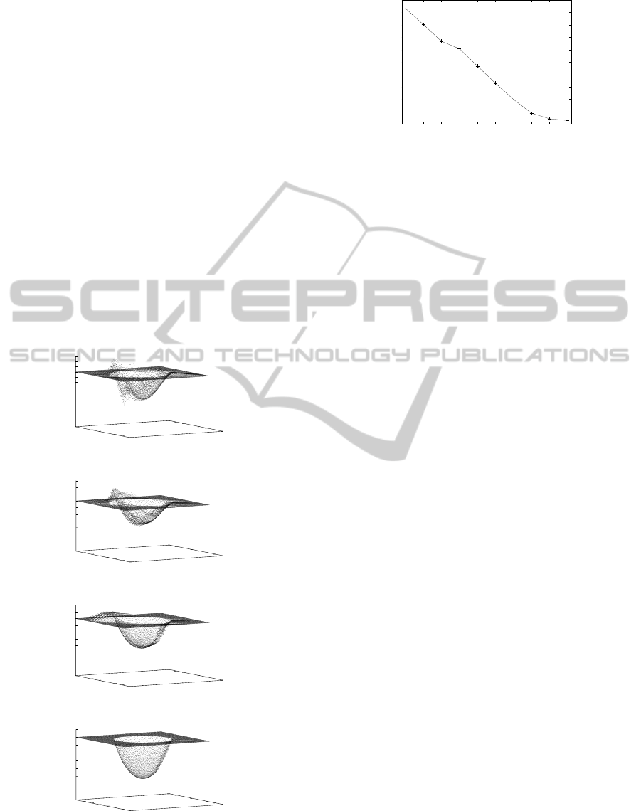
The recovered surfaces are shown in Fig. 2 for the
each repetition of minimization. Figure 3 shows the
RMSEs of the recovered surface with respect to the
repetition number. From these results, the proposed
method can be used repeatedly for recovering the ac-
curate surface with stable computation.
(a)
0
20
40
60
80
100
120
140
0
20
40
60
80
100
120
140
6.2
6.25
6.3
6.35
6.4
6.45
6.5
6.55
6.6
6.65
z
x
y
z
(b)
0
20
40
60
80
100
120
140
0
20
40
60
80
100
120
140
6.1
6.2
6.3
6.4
6.5
6.6
6.7
6.8
z
x
y
z
(c)
0
20
40
60
80
100
120
140
0
20
40
60
80
100
120
140
6
6.1
6.2
6.3
6.4
6.5
6.6
6.7
z
x
y
z
(d)
0
20
40
60
80
100
120
140
0
20
40
60
80
100
120
140
6
6.1
6.2
6.3
6.4
6.5
6.6
z
x
y
z
Figure 2: Recovered surfaces by proposed method: (a) rep-
etition number is 1; (b) 2; (c) 5; (d) 10.
0
0.005
0.01
0.015
0.02
0.025
0.03
0.035
0.04
0.045
0.05
1 2 3 4 5 6 7 8 9 10
RMSE OF DEPTH
ITERATION
Figure 3: RMSE of recovered surface with repetition num-
ber of proposed minimization.
5 CONCLUSIONS
We propose a direct depth recovery method from
shading information, which can be applied to the per-
spective projection. In this method, the representa-
tion of the surface gradient is approximated to avoid
the complicated computation, which is caused by the
straight-forward extension of the parallel projection
method. Through numerical evaluations, we con-
firmed that the repeated application of our minimiza-
tion method can recover a good surface.
REFERENCES
Brooks, M. J. and Horn, B. K. P. (1985). Shape and source
from shading. In proc. Int. Joint Conf. Art. Intell.,
pages 18–23.
Bruhn, A. and Weicke, J. (2005). Locas/kanade meets
horn/schunk: combining local and global optic flow
methods. Int. J. Comput. Vision, 61(3):211–231.
Horn, B. K. P. (1990). Height and gradient from shading.
Int. J. Computer Vision, 5(1):37–75.
Lazaros, N., Sirakoulis, G. C., and Gasteratos, A. (2008).
Review of stereo vision algorithm: from software to
hardware. Int. J. Optomechatronics, 5(4):435–462.
Leclerc, Y. G. and Bobick, A. F. (1991). The direct com-
putation of height from shading. In proc. CVPR ’91,
pages 552–558.
Press, W. H., Flannery, B. P., Teukolsky, S. A., and Vetter-
ling, W. T. (1986). Numerical methods, the art of sci-
entific computing. Cambridge U. Press, Cambridge,
MA.
Simoncelli, E. P. (1999). Bayesian multi-scale differential
optical flow. In Handbook of Computer Vision and
Applications, pages 397–422. Academic Press.
Szeliski, R. (1991). Fast shape from shading. CVGIP: Im-
age Understanding, 53(2):129–153.
Terzopoulos, D. (1983). Multilevel computational pro-
cesses for visual surface reconstruction. Computer Vi-
sion, Graphics, and Image Processing, 24:52–96.
Zhang, R., Tsai, P.-S., Cryer, J. E., and Shah, M. (1999).
Shape from shading: A survey. IEEE Trans. PAMI,
21(8):690–706.
VISAPP 2012 - International Conference on Computer Vision Theory and Applications
448