
A GREAT CIRCLE ARC DETECTOR
IN EQUIRECTANGULAR IMAGES
Seon Ho Oh and Soon Ki Jung
School of Computer Science and Engineering, College of IT Engineering, Kyungpook National University,
80 Daehak-ro, Buk-gu, Daegu 702-701, Republic of Korea
Keywords:
Line Segment Detection, Equirectangular Images, Great Circle Arc Detection, Number of False Alarms.
Abstract:
We propose a great circle arc detector in a scene represented by an equirectangular image, i.e. a spherical image
of the 360
◦
longitude and 180
◦
latitude field of view. Since the straight lines appears curved in equirectangular
images, the standard line detection algorithm cannot be used directly in this context. We extend the LSD
method (Gioi et al., 2010) to deal with the equirectangular images instead of planar images. So the proposed
method has most of the advantages of the LSD method, which gives accurate results with a controlled number
of false detections but requires no parameter tuning. This algorithm is tested and compared to other algorithm
on a wide set of images.
1 INTRODUCTION
Spherical panoramas are increasingly popular so that
the web services such as Flickr enable sharing of this
kind of photos. The development of computational
photography techniques such as stitching and com-
posing makes it easy for people to create the spherical
panoramas. Furthermore, many map services such as
Google Street View provide a 360-degree street-level
view which allows us to explore places around the
world. Accordingly, many conventional image pro-
cessing techniques will be adopted into the panoramic
scene.
Line segment detection is a classical problem
in computer vision. A typical method first applies
Canny’s edge detector (Canny, 1986) followed by the
Hough transform (Ballard, 1981) for extracting all
lines that contain a number of edge points exceeding a
threshold. These lines are thereafter cut into line seg-
ments by using gap and length thresholds. However,
the line detection methods based on Hough transform
are suffering from some problems. First, a high den-
sity of edge points such as textured zones gives many
false detections. Second, it is hard to find a good
threshold. To overcome these problems, various re-
searches were conducted. Burns et al. introduced a
method to use only gradient orientations (Burns et al.,
1986). Desolneux et al. proposed a method to control
the number of false positives (Desolneux et al., 2000).
And then, von Gioi et al. proposed Line Segment De-
tector (LSD), which is an improved method that com-
bines the methods of Burns et al. and Desolneux et al.
(Gioi et al., 2010). However, it cannot be directly ap-
plied to panorama case in which straight lines of the
scene usually appear curved.
Line segment detections for the panoramic images
are proposed by several researchers. Fiala and Basu
introduced the panoramic Hough transform on the pa-
rameter space in 2D for a panoramic-catadioptric im-
age (Fiala and Basu, 2002). They mapped the edge
pixels to panoramic Hough parameter space and then
extracted lines same as standard Hough transform.
Sacht et al. also proposed a method to detect lines
in equirectangular images (Sacht et al., 2010). The
key idea for this method is to use perspective projec-
tion that preserves the line features, and Hough trans-
form with local analysis. They project the viewing
sphere onto the unit cube and apply the bilateral fil-
ter. Thereafter, they perform local analysis proposed
by Szenberg (Szenberg, 2001) to avoid the problems
of Hough transform and discard the cells where no
predominant direction. However, both methods are
based on the Hough transform. Therefore, they can-
not be free from the problems of Hough transform as
mentioned before.
The aim of this paper is to present an effective al-
gorithm that cumulates most of the advantages of the
previous line detection algorithm on the planar image
and extends it to equirectangular images. We choose
LSD proposed by von Gioi et al. because the method
346
Ho Oh S. and Ki Jung S..
A GREAT CIRCLE ARC DETECTOR IN EQUIRECTANGULAR IMAGES.
DOI: 10.5220/0003856303460351
In Proceedings of the International Conference on Computer Vision Theory and Applications (VISAPP-2012), pages 346-351
ISBN: 978-989-8565-03-7
Copyright
c
2012 SCITEPRESS (Science and Technology Publications, Lda.)
made a breakthrough in the extraction of the line seg-
ments. To do this, we first introduce a new represen-
tation of a great circle arc which means a line segment
on the equidistance image. With this representation,
we determine the line-support region and associate it
with a line segment.
The remainder of the paper is organized as fol-
lows. In Section 2, we introduce the geometry of line
segments projected on equirectangular images. Sec-
tion 3 describes how to extend the LSD method for
the equirectangular images. Some experimental re-
sults are illustrated in Section 4. Finally, we describe
the conclusion and future work in Section 5.
2 GREAT CIRCLE ARCS IN
EQUIRECTANGULAR IMAGES
In the photography, a panorama is a broad term for
an image with elongated field of view. Its format
is defined by the projection of a 3D spherical globe
into a 2D image. Two main formats are widely
used; equirectangular and cubic, but we focus on the
equrectangular images in the paper.
Prior to explain the equirectangular projection, we
briefly describe the cylindrical equidistant projection,
whose transformation equations are
x = (λ −λ
0
)cosφ
1
,
y = φ,
(1)
and the inverse formulas are
φ = y,
λ = λ
0
+ x secφ
1
,
(2)
where λ is the longitude, λ
0
is the central meridian
of the projection, φ is the latitude, and φ
1
is the stan-
dard parallels (north and south of the equator) where
the scale of the projection is true. An equirectangu-
lar projection is a cylindrical equidistant projection, in
which the horizontal and vertical coordinates are the
longitude and the latitude, respectively, so the stan-
dard parallel is taken as φ
1
= 0 (Weisstein, 2011).
In general, a line segment can be defined as a
straight region where many of its points share roughly
the same image gradient angle. However, the points
on a a great circle arc in the equirectangular image do
not share the image gradient. Accordingly, we can-
not use the image gradient angle directly. Even so,
there is a geometric relationship related to the image
gradient angle.
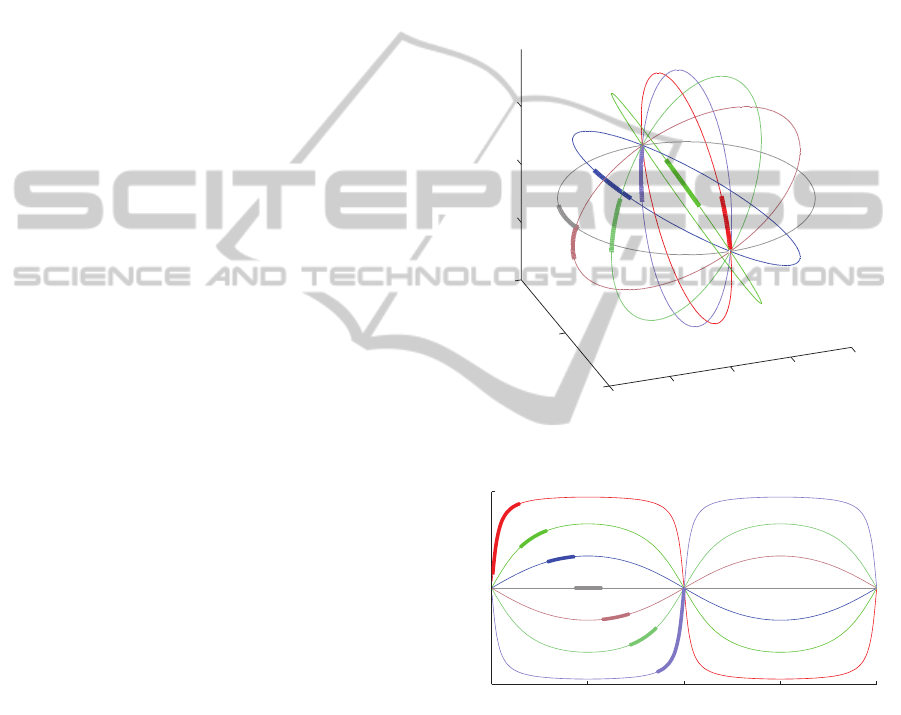
In the spherical panoramic imaging, a 3D point is
projected into a point on the unit sphere where the
center of projection is the center of the sphere. Simi-
larly, a 3D line segment is projected to its correspond-
ing arc segment on a great circle of the unit sphere.
Finally, the arc on a great circle forms a curve seg-
ment in the equirectangular image as shown in Fig. 1.
Thick arcs on the great circles are given as in Fig. 1
(a), and their corresponding curve segments are illus-
trated in Fig. 1 (b). As shown in Fig. 1 (a), a great
circle is defined by the normal vector for the plane
passing through the center of the sphere and the great
circle.
−1
0
1
−1
−0.5
0
0.5
1
−0.5
0
0.5
Y
X
Z
(a) The arcs on the great circle of the unit sphere.
θ
φ
π/2
0
−π/2
0
π/2 π 3/2π 2π
(b) The curve segments on the curve in the equirectangular
image.
Figure 1: The relationship between the arc on the great cir-
cle of the unit sphere and the curve segments in the equirect-
angular image.
With the relationship described above, it is pos-
sible to recover the normal vector for a great circle
(NGC) from the pixel and its level-line angle. In addi-
tion, the points on the arc share the same NGC. There-
fore, it is able to define the arc on the great circle of
the unit sphere (which corresponds to the 3D line seg-
ment in the scene) with its center, length, and NGC.
A GREAT CIRCLE ARC DETECTOR IN EQUIRECTANGULAR IMAGES
347

This representation is what we call the great circle arc
(GCA) and the details will be described in Section
3.3.
3 ALGORITHM
In this section, we explain the algorithm to detect
great circle arcs (GCAs) in equirectangular images.
First we overview the complete algorithm and then
explain the details.
3.1 Overview
Our algorithm extracts GCAs in three steps; region
growing, GCA approximation, and validation. Algo-
rithm 1 describes the pseudo code for the proposed
algorithm. There are three parameters: ρ, τ, and ε.
The parameter ρ is a threshold that the points whose
gradient magnitudes are smaller than ρ are not consid-
ered as seeds of region growing in order to cope with
the quantization effect of image intensity values (Gioi
et al., 2010; Desolneux et al., 2002). And τ is the
angle tolerance used in the search for GCA-support
regions. A small value is more restrictive, leading to
an over-partition of line segments, and a large value
causes unexpected merging of unrelated one. The last
parameter ε is not a critical one; one can safely set its
value to 1 once for all. See (Gioi et al., 2008).
Algorithm 1: GCA detector.
input: An image I, three parameters ρ, τ and ε.
output: A list out of lines in equirectangular images.
1: (LLAngles, GradMod, OrderedListPixels) ←
Grad(I, ρ)
2: Status(allpixels) ← NotUsed;
3: foreach pixel p in OrderedListPixels do
4: if Status(p) = NotUsed then
5: region ← RegionGrow(p, τ, Status);
6: gca ← GCAApprox(region);
7: nfa ← NFA(gca);
8: (nfa, region) ← ImproveGCA(gca);
9: if nfa < ε then
10: Add gca to out;
11: Status(region) ← Used;
12: end
13: end
14: end
The subroutine Grad computes the image gradi-
ent and gives three outputs: the level-line angles, the
gradient magnitude, and an ordered list of pixels. The
pixels are classified into bins by their gradient magni-
tudes.
The list starts with the pixels belonging to the bin
with the highest gradient magnitude and is roughly or-
dered with decreasing gradient magnitude. Status is
used to keep track of pixels used by GCA-support re-
gions. Starting from the first pixels in the list, Region-
Grow is used to obtain a GCA-support region. Then,
GCAApprox gives a GCA approximation of the region
and NFA computes the number of false alarms (NFAs)
of the GCAs. The routine ImproveGCA tries several
perturbations to the initial approximation in order to
get a better approximation.
3.2 GCA-support Regions
Each region starts with just one pixel and it’s NGC is
computed with the level-line angle and the (θ, φ) co-
ordinate of the pixel. Then, the pixels adjacent to the
region are tested; the pixels whose NGCs are equal to
the NGC of the region (ngc
region
) up to a certain preci-
sion are added to the region, and their status is marked
as Used. For each iteration, the NGC of the region is
updated with the mean of NGCs for all pixels in the
region. This process is repeated until no new pixel is
added. The pseudo code is illustrated in Algorithm 2.
Algorithm 2: Region growing.
input: A starting pixel (x, y), an angle tolerance τ,
and Status where pixels used by other regions are
marked.
output: A list Region of pixels.
1: Region ← (x, y);
2: ngc
region
← ComputeNGC(x, y,
LevelLineAngle(x, y));
3: ngc
acc
← ngc
region
4: foreach pixel p in Region do
5: foreach ¯p neighbor of p and Status( ¯p) 6= Used
do
6: ngc
¯p
← ComputeNGC( ¯p.x, ¯p.y,
LLAngle( ¯p.x, ¯p.y));
7: if ngc
¯p
·ngc
region
> cos(τ) then
8: Add ¯p to Region;
9: Status( ¯p) ←Used;
10: ngc
acc
← ngc
acc
+ ngc
¯
P
;
11: ngc
region
← normalize(ngc
acc
);
12: end
13: end
14: end
The subroutine ComputeNGC computes the nor-
mal of the great circle passing through the given pixel,
whose tangential vector is its level-line angle.
In LSD (Gioi et al., 2010), τ is the angle tolerance
used in the search for line-support regions. And it is
also used to set the first angle tolerance used in the
VISAPP 2012 - International Conference on Computer Vision Theory and Applications
348
NFA computation. However, we do not use level-line
angle to determine GCA-support region directly. So
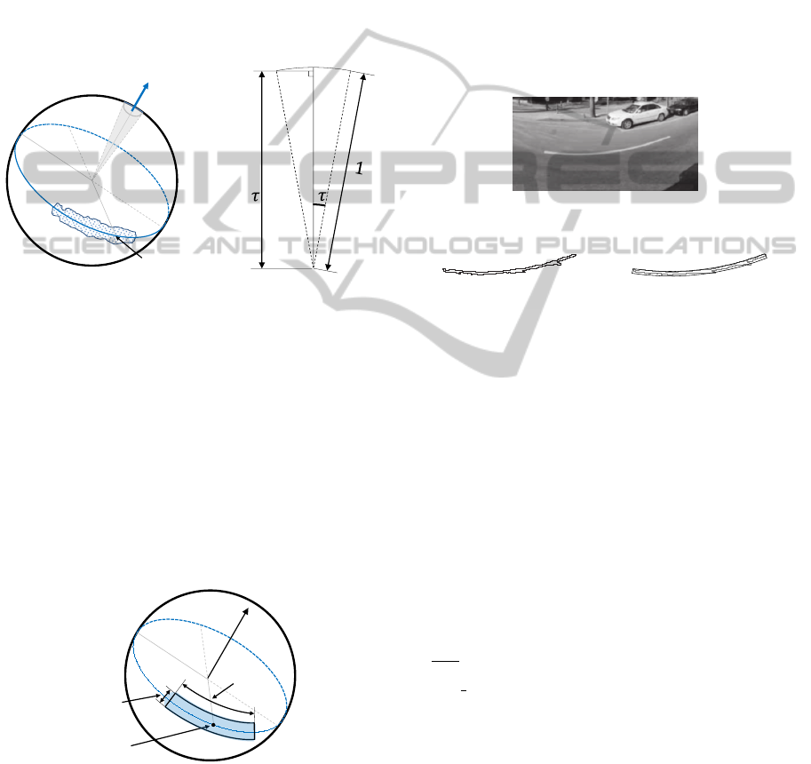
we define a new criterion to determine GCA-support
region. Assume that the GCA-support region is given
and its projection to a unit sphere is shown in Fig.
2. Then, the NGCs of the points in the region form
a gray cone whose opening angle is τ. In this man-
ner, we define cos(τ) as a new criterion to determine
GCA-support region. So that all NGCs of points in
the GCA-support region are laid in the cone. In other
words, only the pixels whose the inner product with
ngc
region
is greater than cos(τ) are considered.
cos
GCA-support region
mean of NGC
Figure 2: Region growing criteria defined by angle toler-
ance τ.
3.3 GCA Approximation of Regions
Prior to the validation step, it is necessary to simplify
the GCA-support region (a set of pixels) to a GCA (a
geometrical object). In general, a line support region
in a planar image can be represented by a rectangle.
However, a GCA-support region in an equirectangu-
lar image is bounded by a curved region. So we de-
fine a GCA with its center, length, width, and NGC as
shown in Fig. 3.
Center
NGC
Length
Width
Figure 3: GCA is characterlized by a region determined by
its center point, NGC, length and width.
In order to obtain a GCA, the center of the GCA-
support region should be determined first. In our al-
gorithm, the center of mass is used to compute the
center of the GCA-support region, and the gradient
magnitude is used as the mass of the pixels, just like
von Gioi et al. did. NGC is computed in three steps:
1. Project all the points in the GCA-support region
to unit sphere.
2. Compute the initial NGC with plane fitting
method.
3. Compensate NGC to satisfy that its associated
plane is passing through the center of GCA.
The length and the width are chosen to cover the
GCA-support region. Both are angular values since
GCA is defined on the unit sphere. Fig. 4 shows an
example of the result.
(a) A part of input image.
(b) A GCA-support region. (c) A GCA approximation.
Figure 4: Example of a GCA approximation of a GCA-
support region.
3.4 Validation of GCAs
Like von Gioi et al.’s, the validation step in our algo-
rithm is also based on the a contrario approach and
the Helmholtz principle proposed by Desolneux et al.
(Desolneux et al., 2000; Desolneux et al., 2008). The
detection can be considered as a hypothesis testing
problem.
There are many tests T
gca
as there are potential
GCAs in the equirectangular image. Similar to rect-
angle cases, there are (NM)
2
potential GCAs, start-
ing and ending on a point of the grid Γ. If we accept
√
NM possible width values for the GCAs, this gives
(NM)
5
2
tests.
Following the LSD (Gioi et al., 2010), we define
the Number of False Alarms of gca ∈ T
gca
and an im-
age i, as
NFA(gca, i) = #T
gca
·P
H
0
[k(gca, I) ≥ k(gca, i)], (3)
where P
H
0
is the probability on the a contrario model
H
0
, I is a random image on H
0
, #T
gca
is the num-
ber of potential GCAs in the image, and the statis-
tics k(gca, x) denotes the number of aligned points
in the GCA gca and image x. In other words, NFA
A GREAT CIRCLE ARC DETECTOR IN EQUIRECTANGULAR IMAGES
349
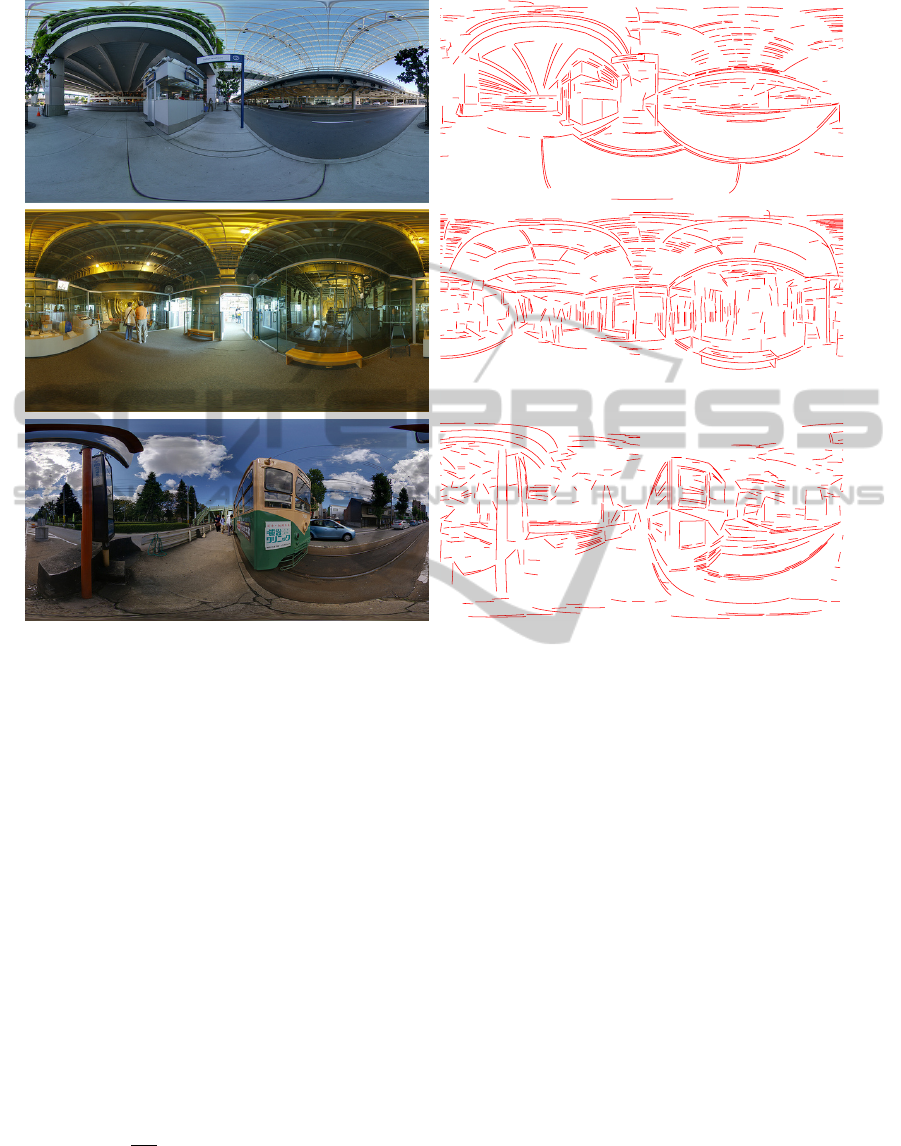
Figure 5: Result of our algorithm on internet images (Flicker, 2011).
value is the expected number of detection on the
non-structured model. Therefore, the smaller the
NFA(gca, i) value, the more meaningful gca is, i.e.,
the less likely it is to appear in an image drawn from
the H
0
. We reject H
0
if and only if NFA(gca, i) ≥ ε
gives.
The method is justified in the same way as von
Gioi et al., i.e., the expected number of detection on
the non-structured model is less than ε, which gives
back the Helmholtz principle. And the dependence of
the method on ε is very week. For more details, see
(Desolneux et al., 2000). In our experiment, we fix
ε = 1 once for all.
4 RESULTS
All the experiments were done without tuning any pa-
rameter at all. In our experiments, τ is 22.5
◦
, ε is 1,
and ρ is given as
q
sinτ
where q is the norm of quanti-
zation noise (for more details, see (Gioi et al., 2010;
Desolneux et al., 2002)).
Fig. 5 shows a series of experiments on the in-
ternet images. The images on the left column are the
input images, and the ones on the right column are
the results of the proposed algorithm. As you can
see in the results, almost all of the expected GCAs
are found, except some small ones. And there are
very few false detections. Some images contain non-
geometrical contents, such as vegetation or cloud, and
they do not correspond to real straight or flat objects
as shown in the third image of Fig. 5. However, it
is a reasonable interpretation in terms of the structure
present on the image at a given resolution. The re-
sults illustrated in Fig. 5 are acceptable in the sense
that every detection corresponds to a locally straight
structure in the equirectangular image.
Fig. 6 shows a comparison of our algorithm with
Sacht et al.’s method for two images. The first row
shows input images with magnified region to see the
results in detail. The middle and the bottom rows il-
lustrates the results of Sacht et al. method and the
proposed algorithm, respectively.
In the result of Sacht et al.’s method, there are
many undetected line segments. In addition, it has
much false detection. On the other hand, the result
of the proposed algorithm represents well the over-
all structure of the scene. In addition, the lines that
VISAPP 2012 - International Conference on Computer Vision Theory and Applications
350
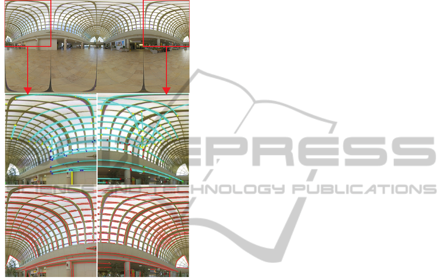
were not detected in Sacht et al.’s were detected well.
However, our algorithm also has several false detec-
tions. This is because a given image is similar to the
tunnel and it contains many curves.
Figure 6: Comparison of two methods: Sacht et al. (middle)
and the proposed algorithm (bottom).
5 CONCLUSIONS
In this work, we presented a GCA detector in the
equirectangular images. The key idea of our algo-
rithm is to represent the line segments in the equirect-
angular image as GCAs. With this representation, we
can define the GCA-support region and approximate
geometrical object, which associated with a line seg-
ment. Finally, we successfully extend the LSD algo-
rithm, while maintaining most of its advantages. The
proposed algorithm gives accurate results and a con-
trolled number of false detections, without any param-
eter tuning for each image.
Although the proposed algorithm inherits a set
of good features from the original LSD method, the
computation of k(gca, i) and n(gca) are more com-
plicated than the rectangular case. To make things
worse, the effect of noise is also critical for the pro-
posed algorithm as von Gioi et al. noted.
To address the limitations of our work, we intent
to carefully consider the validation stage. In addi-
tion, the computation of NFA still has to be improved.
Thus, quantative and qualitative analysis of false de-
tection would be done. Also, we will analyze the ef-
fect of noise in equirectangular images.
ACKNOWLEDGEMENTS
This research was supported by Basic Science Re-
search Program through the National Research Foun-
dation of Korea (NRF) funded by the Ministry of Ed-
ucation, Science and Technology (2011-0006132).
REFERENCES
Ballard, D. (1981). Generalizing the hough transform to de-
tect arbitrary shapes. Pattern Recognition, 13(2):111
– 122.
Burns, J. B., Hanson, A. R., and Riseman, E. M. (1986). Ex-
tracting straight lines. IEEE Transactions on Pattern
Analysis and Machine Intelligence, 8:425–455.
Canny, J. (1986). A computational approach to edge de-
tection. IEEE Transactions on Pattern Analysis and
Machine Intelligence, 8:679–698.
Desolneux, A., Ladjal, S., Moisan, L., and Morel, J.-M.
(2002). Dequantizing image orientation. IEEE Trans-
actions on Image Processing, 11(10):1129–1140.
Desolneux, A., Moisan, L., and Morel, J. (2008). From
Gestalt theory to image analysis: a probabilistic
approach. Interdisciplinary applied mathematics.
Springer.
Desolneux, A., Moisan, L., and Morel, J.-M. (2000). Mean-
ingful alignments. International Journal of Computer
Vision, 40(1):7–23.
Fiala, M. and Basu, A. (2002). Hough transform for feature
detection in panoramic images. Pattern Recognition
Letters, 23:1863–1874.
Flicker (2011). Flickr: Equirectangular.
http://www.flickr.com/groups/equirectangular/.
Gioi, R. G. V., Jakubowicz, J., Morel, J.-M., and Randall,
G. (2008). LSD: A line segment detector. Technical
report.
Gioi, R. G. V., Jakubowicz, J., Morel, J.-M., and Randall,
G. (2010). LSD: A fast line segment detector with a
false detection control. IEEE Transactions on Pattern
Analysis and Machine Intelligence, 32:722–732.
Sacht, L. K., Carvalho, P. C., Velho, L., and Gattass, M.
(2010). Face and straight line detection in equirect-
angular images. In Proceedings of Workshop of Com-
puter Vision (WVC).
Szenberg, F. (2001). ACOMPANHAMENTO DE CENAS
COMCALIBRAO AUTOMTICA DE CMERAS. PhD
thesis, PUC-Rio. PhD thesis, PUC-Rio.
Weisstein, E. W. (2011). Equirectangular projection.
http://mathworld.wolfram.com/EquirectangularProjec
tion.html.
A GREAT CIRCLE ARC DETECTOR IN EQUIRECTANGULAR IMAGES
351
