
GLYPH- AND TEXTURE-BASED VISUALIZATION
OF SEGMENTED TENSOR FIELDS
Cornelia Auer, Claudia Stripf, Andrea Kratz and Ingrid Hotz
Zuse Institut Berlin, Takustrasse 7, 14195 Berlin, Germany
Keywords:
Tensor Field Visualization, Texture Mapping, Glyph Placement.
Abstract:
In this work we show how the variability of visualization methods like textures and glyphs can be used to
enhance established methods like topology. A topology-based segmentation (Auer et al., 2011) serves as
framework to map textures and place glyph exponents for two dimensional symmetric tensor fields. The
textures encode physical properties of the underlying field and support the understanding of the field as a
whole, whereas the glyph exponents can be used to give detailed insight at distinctive locations.
1 INTRODUCTION
Where to Place which Information and how? This
is a crucial question even experts in visualization are
permanently confronted with. An incomplete view
is as undesirable as a cluttered image. Topological
methods have a long tradition and for domain experts
they serve as visualization itself. However, for un-
trained users this might be too abstract – especially
if the visualization is meant to support a first under-
standing of the data. In this work, we exploit the
topology-based segmentation of a two-dimensional
tensor field (Auer et al., 2011) as basis for texture
generation, as well as for the placement of glyphs.
Textures are a powerful tool to design continu-
ous visualizations. They offer many parameters that
can be used to encode features of interest. This
makes textures especially interesting for the visual-
ization of tensor fields. Tensor fields contain direc-
tional and scalar features which can be encoded in
texture parameters. One challenge for many texture-
based methods is the definition of appropriate tex-
ture coordinates. This is accomplished by the cells of
the topology-based segmentation; they serve as con-
sistent framework for the texture mapping. A dense
visualization of the underlying tensor field can be
generated using every pixel of the image to convey
physical properties of the field. Furthermore, a di-
versity of visualization options arises: To encode di-
rectional information, for example, stripe patterns can
be used; but also knitting or basketwork patterns are
presented and evaluated towards their applicability to
depict central tensor properties within the segmentat-
ion framework. The goal hereby is not to display all
possible features in one image but to offer a flexible
framework to a user to switch views for the different
points of interest.
The placement of glyphs is an intricate topic for
vector as well as tensor visualization. Here, we use
the tensor field segmentation to display glyphs at dis-
tinctive locations in the given cells. The advantages
of the global structural information provided by the
topology and the detailed depiction of representative
tensors via glyphs are combined in a single image.
Tensors are of interest in many application fields,
for example, engineering, physics but also computer
graphics. Especially for tensors in physics and engi-
neering, even for two dimensional fields, the develop-
ment of expressive visualizations is still an ongoing
research topic. We will demonstrate our results for
stress tensors which are of high importance in me-
chanical engineering.
2 RELATED WORK
The focus of this review is on visualization meth-
ods designed for tensor fields arising in applications
such as physics and mechanical engineering. In gen-
eral, the developed visualization methods can be sub-
divided into local and continuous methods.
Local Methods. Local methods use geometric ob-
jects (glyphs) to depict single tensors at discrete
points. Shape, size, color, and texture can be used
to encode tensor properties. The most common glyph
670
Auer C., Stripf C., Kratz A. and Hotz I..
GLYPH- AND TEXTURE-BASED VISUALIZATION OF SEGMENTED TENSOR FIELDS.
DOI: 10.5220/0003857106700677
In Proceedings of the International Conference on Computer Graphics Theory and Applications (IVAPP-2012), pages 670-677
ISBN: 978-989-8565-02-0
Copyright
c
2012 SCITEPRESS (Science and Technology Publications, Lda.)
for tensors is an ellipsoid alligned to the tensor’s
eigenvectors and scaled according to its eigenvalues
(Figure 1). Beside the design of glyphs (see (Hashash
et al., 2003) for an overview of glyphs for stress and
strain tensors), perceptional issues such as visual am-
biguity need to be solved (Schultz and Kindlmann,
2010) when using glyphs for visualization. Another
challenge is the placement of glyphs to maximize the
information that is conveyed in an image. Previous
methods in this context aimed to create sample dis-
tributions that avoid holes and overlaps (Kindlmann
and Westin, 2006), (Hlawitschka et al., 2007), (Feng
et al., 2008), (Kratz et al., 2011). In this work, we ad-
dress the question where to place glyphs by exploiting
a segmentation of the tensor field.
Continuous Methods. Closely related to our work
are texture-based methods, which are motivated by
vector field visualization. Line integral convolu-
tion (LIC) (Cabral and Leedom, 1993), for example,
has been extended to HyperLIC (Zheng and Pang,
2003). It uses a multi-pass approach to represent
the orientation of one eigenvector field and to high-
light anisotropy. Another extension are fabric tex-
tures (Hotz et al., 2004). Two LIC images for every
eigenvector field are computed and blended, which
leads to an image that resembles a fabric encoding
central physical properties of stress tensor fields into
fiber thickness (thin = compression, thick = expan-
sion). Recently, a novel method based on anisotropic
sampling was introduced (Kratz et al., 2011). By
computing a generalized Voronoi diagram on the ba-
sis of a tensor-determined local metric, the result-
ing regions can be texturized which results in a large
variety of possibilites to create visualizations. In
general, texture-based methods are restricted to two-
dimensional surfaces.
Three-dimensional visualization methods for
stress tensor fields are rare (Dick et al., 2009), (Kratz
et al., 2011). They focus on hybrid methods to em-
phasize interesting regions and to avoid clutter. When
features of interest are not known in advance, explo-
rative methods can help (Kratz et al., 2011). To depict
the behavior of a single eigenvector field, tensorlines
can be used. These are defined as lines that are tan-
gential to the chosen eigenvector field. Hyperstream-
lines (Delmarcelle and Hesselink, 1993) are an exten-
sion, which additionally incorporate the eigenvalues
and other principal directions.
Topological Methods. Tensor fields can also be
represented by extracting their topology, which is
represented by a graph structure. This topological
graph consists of degenerate points and connecting
tensorlines (Delmarcelle, 1994), (Lavin et al., 1997),
which separate the field into regions of similar eigen-
vector behavior. Simplification and tracking of the
graph (Tricoche et al., 2001) results in a structure
that is easier to understand and enhances their prac-
tical applicability. This paper builds on a topologi-
cal segmentation (Auer et al., 2011). Therefore, the
topological graph is extracted (Sreevalsan-Nair et al.,
2010) and recursively refined according to eigen-
value characteristics. Thus, a segmentation of the
field is achieved that accounts for both, eigenvalue
and eigenvector behavior. Work that is concerned
with topology extraction for three-dimensional fields
is rare (Hesselink et al., 1997), (Zheng and Pang,
2004), (Tricoche et al., 2008).
3 BASICS AND NOTATION
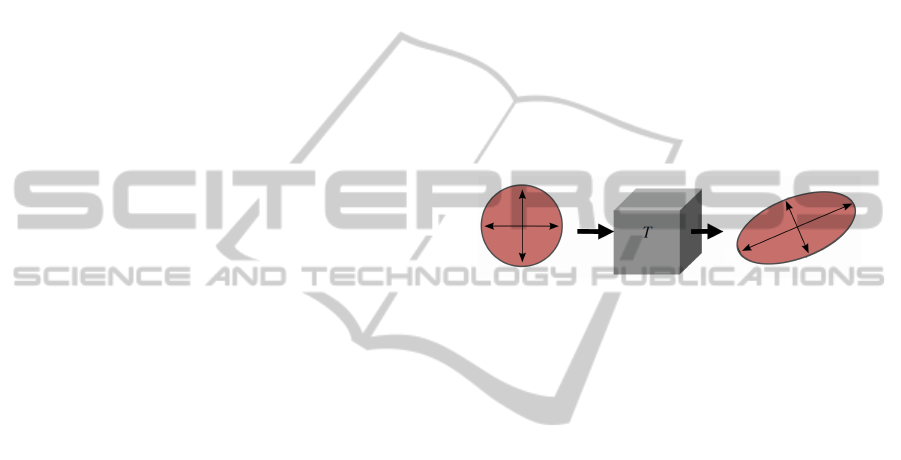
Figure 1: Illustration of the tensor concept: result (ellipse)
of applying a tensor to an isotropic element (sphere). The
resulting eigenvectors are depicted as arrows and the eigen-
values are reflected by the scaling of the arrows.
3.1 Tensors
This work focuses on the visualization of two-
dimensional symmetric tensors. For a fixed coordi-
nate system in R
2
such a tensor can be described as
2 × 2 matrix of real numbers. For the remainder of
this paper, if not stated differently, the word tensor
refers to two-dimensional symmetric tensors.
Eigenvalues λ
i
∈ R and eigenvectors
↔
v
i
∈ R
2
, with
i = 1, 2 are important invariants of a tensor. They
are defined by the characteristic equation T · λ
i
=
↔
v
i
· λ
i
. The eigenvectors specify the direction of ex-
tremal variation of the quantity encoded by the ten-
sor; the eigenvalues give the magnitude of those ex-
tremal variations (Figure 1). For symmetric tensors
the eigenvalues are real and the eigenvectors mutually
orthogonal. The double arrows allude to the fact that
eigenvectors are bidirectional. A tensor is fully repre-
sented by its eigenvectors and eigenvalues. In the fol-
lowing the eigenvalues are ordered such that λ
1
≥ λ
2
.
They are called major respectively minor eigenvalues
with associated major and minor eigenvector.
3.2 Tensor Fields
A tensor field assigns a tensor to each point in a do-
main. In our case the input tensor fields are given on
GLYPH- AND TEXTURE-BASED VISUALIZATION OF SEGMENTED TENSOR FIELDS
671

a triangulated planar domain, where each vertex of
the triangulation is assigned to a tensor. The tensor
fields are decomposed into to two eigenvector- and
two eigenvalue fields (major resp. minor). Integral-
lines that are tangential to an eigenvector field every-
where are called tensorlines. To distinguish whether
the tensorlines belong to the major or the minor eigen-
vector field, a color-coding is used: blue refers to the
minor field and red to the major field.
3.3 Topology
The topology is represented by the topological graph,
which consists of degenerate elements and separatri-
ces. Degenerate elements are locations where both
eigenvalues are equal, λ
1
=λ
2
, and thus the eigenvec-
tors
↔
v
i
are not uniquely defined. Mostly they occur
as points but also as elements of higher dimensional-
ity, such as lines. Separatrices are distinctive tensor-
lines, that radially emerge from degenerate elements
and bound sectors of homogeneous eigenvector be-
havior. For more details we refer to (Delmarcelle and
Hesselink, 1993).
4 TOPOLOGICAL
SEGMENTATION
This work builds on a refined topological graph yield-
ing a complete segmentation of the tensor field (Auer
et al., 2011). This segmentation returns cells with
homogeneous eigenvector and eigenvalue behavior.
Starting point for the segmentation is the integral
topological graph combining the topology of both
eigenvector fields. As the eigenvector fields are or-
thogonal to each other this graph segments the tensor
field into curvilinear cells of homogeneous eigenvec-
tor behavior (Figure 2(a)). Eigenvalues are used to it-
eratively adapt the topological cells until they fulfill
predetermined resolution, accuracy, and uniformity
criteria (Figure 2(b,c)). If a cell exhibits dissimilarity
above a predefined accuracy threshold, it gets split by
starting a subdividing tensor line. Further, neighbor-
ing cells that are homogeneous get merged by delet-
ing the connecting edge. To steer the similarity of
eigenvalue characteristics within a cell, one or more
expressive scalar fields are defined. These can be the
eigenvalues, but also derived tensor invariants. For
stress tensor fields, e.g., quantities of special interest
arise in context with failure analysis. Exemplary we
use relative shear τ
R
and maximum shear stress τ as
anisotropy measures.
τ =
|
λ
1
− λ
2
|
, and τ
R
=
|
λ
1
− λ
2
|
q
λ
2
1
+ λ
2
2
+ A
2
, (1)
where A ∈ R is a positive constant.
The resulting cells are bounded by tensorlines and
possibly degenerated lines. The integration of the ten-
sor lines using a Runge-Kutta-4th-order integration
scheme yields a representation of tensorlines as poly-
lines. Adaptive step sizes are used to maximize the
accuracy of this numerical integration scheme.
5 VISUALIZATION METHOD
In this work we build upon the results of the seg-
mentation (Section 4) and extend it to a texture- and
glyph-based visualization. Mapping textures into the
segmented cells yields a continuous rendering of the
tensor field. This facilitates a comprehension of the
field’s global nature. The glyph-based approach com-
bines the advantages of the global structural informa-
tion provided by the topology and the local detailed
view of representatives via glyphs.
Cell Structure. Cells that are not adjacent to de-
generate points or the domain boundary are quadran-
gular and bounded by two major and minor tensor-
line segments in alternating order (Figure 2(c),(d)).
Other cells can have more general shapes. The bound-
aries of the extracted cells are stored as polylines (Fig-
ure 3).
Preprocessing. As mentioned in Section 4, the
bounding tensorlines are computed by an integration
scheme with adaptive step size. This guarantees ac-
curate results in the segmentation process but leads to
irregular distances between the vertices of the poly-
lines. To obtain good results for the texturing and
glyph locations, however, a more uniform sampling
of the cell boundaries is favorable. This is achieved
by a pre-processing step deleting respectively adding
vertices if the distance to adjacent vertices does not
fall in a pre-defined distance interval. An angle cri-
terion guarantees that tensorlines are still sufficiently
aligned with the eigenvector fields.
For the texture mapping the segmented cells need
to be triangulated. We use a constrained Delaunay tri-
angulation that maintains non-convex shape.
All pre-processing steps only have to be per-
formed once after the segmentation process.
Eigenvalue Mapping. The goal of this work are in-
tuitive visualizations of stress tensors. These, in gen-
eral, are not positive definite and thus, have positive as
well as negative eigenvalues. We will use the eigen-
values to control basic texture parameters such as tex-
ture density. Therefore the eigenvalues are mapped
IVAPP 2012 - International Conference on Information Visualization Theory and Applications
672
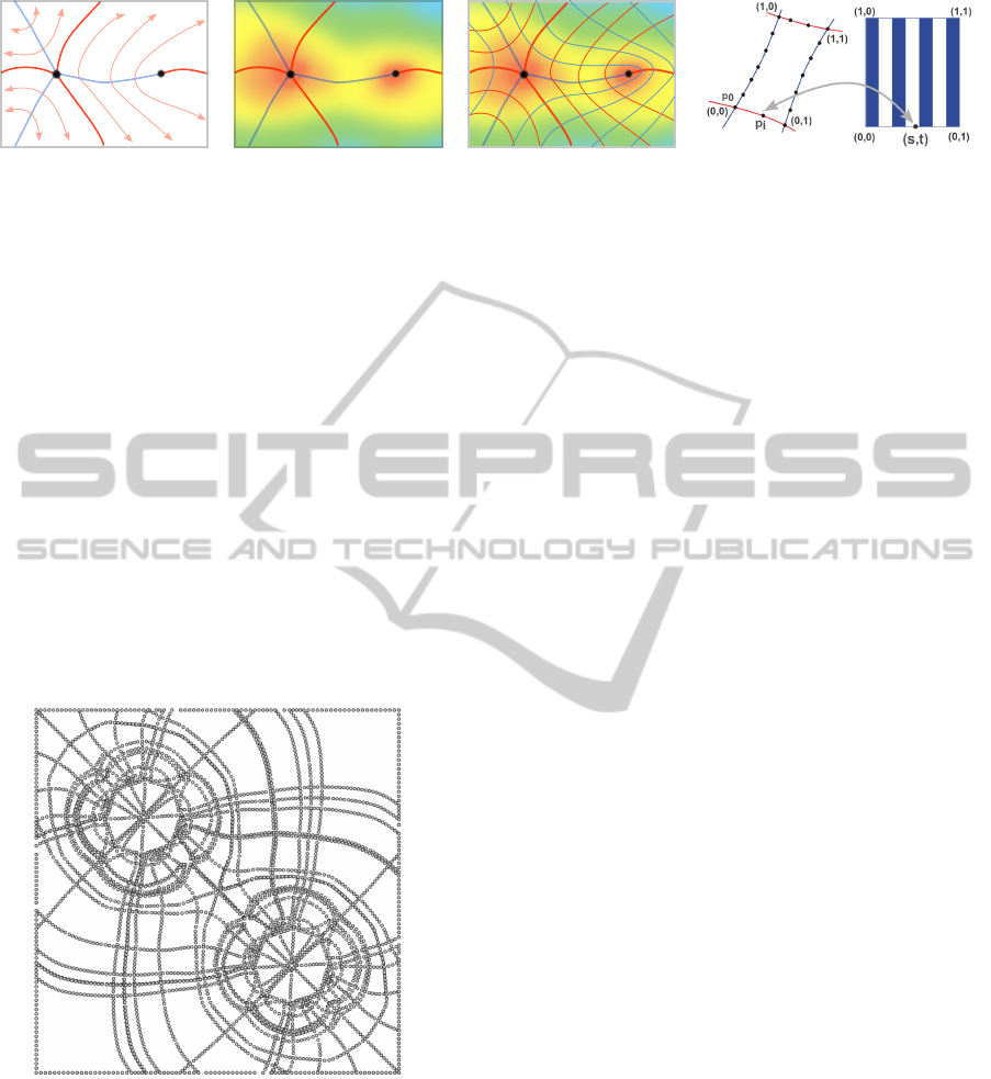
(a) (b) (c) (d)
Figure 2: (a-c) Schematic illustration of the segmentation process. (a) Step 1: Integral topological graph with degenerate
points as black dots, separatrices as bold lines (major in red, minor in blue). The light red lines depict tensorlines within
the segmented regions and exemplarily illustrate how separatrices aggregate homogeneous eigenvector behavior. (b) Step 2:
Definition of scalar field. (c) Step 3: Refinement of topological graph according to scalar field. (d) Texturization of segmented
cell. Mapping of point p
i
to texture coordinate (s, t) in quadrangular cell.
into a restricted positive interval. We adopt a mapping
that simulates a texture deformation generated by the
underlying tensor field (Hotz et al., 2004). Thus,
negative eigenvalues (compression) lead to dense and
positive eigenvalues (expansion) to sparse textures.
Hotz et al. define:
F(λ) = a + σ · f (λ) . (2)
The function f is chosen to have a large slope in the
neighborhood of zero. In this work, f is the hyper-
bolic tangent, which preserves the differentiation of
negative and positive eigenvalues. The parameter a
relates to an offset and σ is an additional scaling fac-
tor for the slope. Both can be adjusted by the user.
Figure 3: Result of a segmentation, points of the cell bound-
ing polylines are depicted as spheres.
5.1 Segmentation-based Glyph
Placement
The characteristics of the tensor field – the eigen-
vectors and eigenvalues – are similar inside each ex-
tracted cell (Section 4). Thus, the essential tensor
properties of each cell can be visualized by one rep-
resentative glyph. The task is to find an appropriate
position within each cell to place this representative.
Since most of the segmented cells are non-convex we
follow an algorithm for the computation of barycen-
troids of arbitrarily shaped planar polygons (Rusta-
mov et al., 2009). This algorithm is based on an in-
terior distance measure. The barycentroid is defined
as the point with minimal average interior distance to
the boundary points. Finding this point is a convex
optimization problem and can be solved by standard
gradient descent routines. The barycentroid has the
characteristic that it captures the semantic center of
the polygon and lies inside any arbitrary shaped pla-
nar polygon. See Figure 5 for results.
5.2 Segmentation-based Texturization
Using the segmented cells as basis for texturization
has several benefits. The cells inherently provide the
parametrization for the texture mapping and the un-
derlying topology ensures structural correctness.
Also the segmented cells bounded by tensorlines
already give the eigenvector directions. Simple pro-
cedural stripe textures already depict one eigenvector
field. Thus, the use of textures with one or two orthog-
onal dominant directions results in continuous repre-
sentations of the correct eigenvector behavior within
these cells (Figure 4). But also more sophisticated
textures, like knitting patterns, lead to expressive rep-
resentations (Figure 7). The density of the texture pat-
tern will also be used to reflect physical properties of
the tensor field, such as compression and expansion
(e.g. Figure 4(b)).
Cells containing degenerate elements in their
boundary can have more complex shapes and the
eigenvector behavior cannot be easily represented by
simple stripe patterns. In addition, in the proxim-
ity of degenerate elements the eigenvector behavior
is weakly expressed. For such cells two options are
provided. Either these cells are skipped or textured
with an isotropic noise pattern encoding information
about the isotropic eigenvalues.
GLYPH- AND TEXTURE-BASED VISUALIZATION OF SEGMENTED TENSOR FIELDS
673

For one-directional textures, as stripe patterns, one
image per eigenvector field is computed. To depict
both eigenvector fields in one image the results for
each field are blended (Figures 4(c), 6).
The texturization is performed by vertex and fragment
shaders. Texture coordinates (s, t), with s, t ∈ [0, 1] for
quadrangular cells are initially computed by mapping
the points of a cell boundary to a unit square (Fig-
ure 2(d)).
5.2.1 Rendering of Eigenvector Directions
All methods that are presented in the following are
based on textures with linelike elements to depict di-
rections. To ensure that the cell size does not affect
the perception of the pattern, we need a special map-
ping approach that provides an approximately con-
stant pattern frequency (Hummel et al., 2010)(Fig-
ure 4(a)). Hummel et al. adjust the sampling fre-
quency according to the image-space partial deriva-
tives η
s
, η
t
at pixel (i, j) of the texture coordinate
(s, t):
η
s
(i, j) =
s
δs
δi
2
+
δs
δ j
2
,
η
t
(i, j) =
s
δt
δi
2
+
δt
δ j
2
.
(3)
The initial texture coordinates (s, t) remain un-
changed. The evaluation of the input texture P is mod-
ified according to the variation of η
s
and η
t
and steers
the pattern frequency in the final image.
ˆ
P
l
s
,l
t
gives
the frequency adjusted texture values
ˆ
P
l
s
,l
t
(s, t) := P(s ·2
−l
s
, t ·2
−l
t
) , (4)
with l
s
= log
2
η
s
and l
t
= log
2
η
t
. Hence, short edges
with high partial derivatives yield a low pattern fre-
quency. For large edges this works vice versa. The
resulting pattern frequency also interactively adjusts
to the current zoom level and resolution of the image.
As resolution levels are discretely defined values for
neighboring resolution levels are computed and bilin-
ear filtering applied to achieve a smooth pattern fre-
quency. The evaluation of Equation 3 can be done by
built-in functionality of the rendering system.
5.2.2 Rendering of Eigenvalue Characteristics
Line Frequency. The approach of Hummel et
al. (Hummel et al., 2010) serves as basis to en-
code physical properties like compression and expan-
sion by the pattern frequency (Figure 4(b)). This is
achieved by replacing Equation 3 by the following:
η
s
(i, j) =
s
δs
δi
·
˜
λ
1
2
+
δs
δ j
·
˜
λ
1
2
,
η
t
(i, j) =
s
δt
δi
·
˜
λ
2
2
+
δt
δ j
·
˜
λ
2
2
,
(5)
where
˜
λ
1
and
˜
λ
2
are the mapped eigenvalues. Thus,
the pattern frequency steers the perception of the field:
in combination with the mapping (Eq. 2) negative
eigenvalues lead to a higher frequency and allude to
compression. Mapped positive eigenvalues cause a
lower frequency which depicts expansion.
Color Mapping. A simple but effective way of con-
veying additional information is to blend color infor-
mation on the input textures (Figures 4(c), 6(a),(b),
and 7(b),(c)). Coloring can be applied to the eigenvec-
tor fields (one color for each field) but also according
to derived scalar measures such as the magnitude of
one eigenvalue, relative shear, maximum shear stress
(Eq. 1), or the determinant (λ
1
· λ
2
).
Blur by Derived Scalar Quantities. If non relevant
information should be suppressed in the final image, a
post-processing step can be applied to the texturized
image. We employ a blur filter, but also the opac-
ity could be modified to hide regions of low informa-
tion content. Again quantities like relative and ab-
solute shear stress come into question (Figures 6(b),
and 7(b),(c)) to steer the post-processing. The pixels
of the texturized image are convolved with a Gaus-
sian kernel, where the size of the kernel is propor-
tional to the respective value of the chosen quantity.
For example, if the blur should be determined with
respect to relative shear, isotropic regions are con-
volved with a larger kernel and anisotropic regions
are convolved with a smaller kernel. Thus, regions
with strongly expressed eigenvector directions are en-
hanced and isotropic regions blurred.
6 RESULTS
In this section, the results of the developed visualiza-
tion approaches are presented and evaluated by means
of two simulated datasets: the one-point load and the
two-point load. The one-point load is a solid block
given as a cubic volume with a single load applied to
it. The two-point load is similar, just that two loads of
opposing sign are applied to it. The two datasets are
generated by a Finite Element Method (FEM). The
methods presented above are analyzed on planar cuts
of the volumetric datasets.
IVAPP 2012 - International Conference on Information Visualization Theory and Applications
674
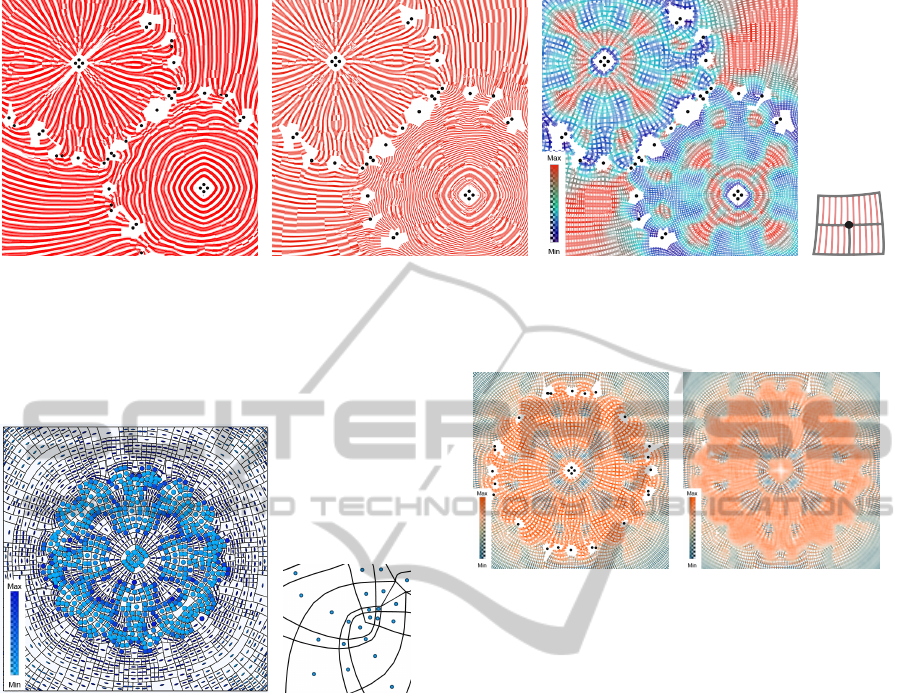
(a) (b) (c) (d)
Figure 4: Data set: Two-point load. Visualization of major eigenvector field (a) with even pattern frequency, (b) with encoded
mapped eigenvalues. (c) Superposition of both eigenvector fields, color by relative shear. (d) Illustration of a hanging node.
6.1 Glyph-based Visualization
(a) (b)
Figure 5: Data set: One-point load. (a) Glyph placement in
the data set. (b) Close-up of pre-computed barycentroids.
Figure 5 shows the results of the segmentation-
based glyph placement (Section 5.1) applied to the
one-point load. The glyphs are placed at the pre-
computed barycentroids, oriented according to the
eigenvectors and scaled by the mapped eigenvalues
(Eq. 2). The color is assigned according to the relative
shear (Eq. 1). Isotropic tensors are encoded in light
blue and spherical geometries. Anisotropic tensors
are encoded in dark blue and result in well-marked
ellipses. This work is not concerned with elaborate
glyph design or similar. With the glyph placement we
rather want to provide a basis for the variety of glyphs
provided in the literature (Section 2). The close-up in
Figure 5(b) nicely shows how the barycentroids cap-
ture the semantic center of non-convex polygons.
6.2 Texture-based Visualization
Figure 4(a) displays the directions of the major
eigenvector field. Here the basic approach of ap-
(a) (b)
Figure 6: Data set: One-point load. (a) Superposition of
both eigenvector fields, color coding according to mapped
eigenvalues; (b) post-processing blur by relative shear.
proximately constant image space line density (Sec-
tion 5.2.1) is applied. Even though the textures are
mapped cell-wise the continuous character of the im-
age is harmonious. Only at transitions of cells with
hanging nodes (Figure 4(d)) slight disruptions are no-
ticeable. Zooming in the image automatically adapts
the texture such that the stripe frequency and the
even appearance is maintained. Figure 4(b) extends
the representation by encoding the physical behav-
ior. The pattern frequency is scaled by the mapped
eigenvalues (Eq. 5). In the lower right corner nega-
tive eigenvalues are predominant and clearly result in
a higher pattern frequency. This resembles to com-
pressive forces and is in contrast to the upper left cor-
ner which is characterized by expansive forces. In
Figure 4(c) the textures for both eigenvector fields are
blended. The pattern frequency is determined again
by Equation 5 and color coding is applied accord-
ing to the relative shear. Isotropic regions are colored
in blue and characterized by an isotropic pattern fre-
quency. In regions of high anisotropy strongly differ-
ing eigenvalues lead to the unequal pattern frequen-
cies for the two eigenvector fields, which is addition-
ally emphasized by the red color.
GLYPH- AND TEXTURE-BASED VISUALIZATION OF SEGMENTED TENSOR FIELDS
675
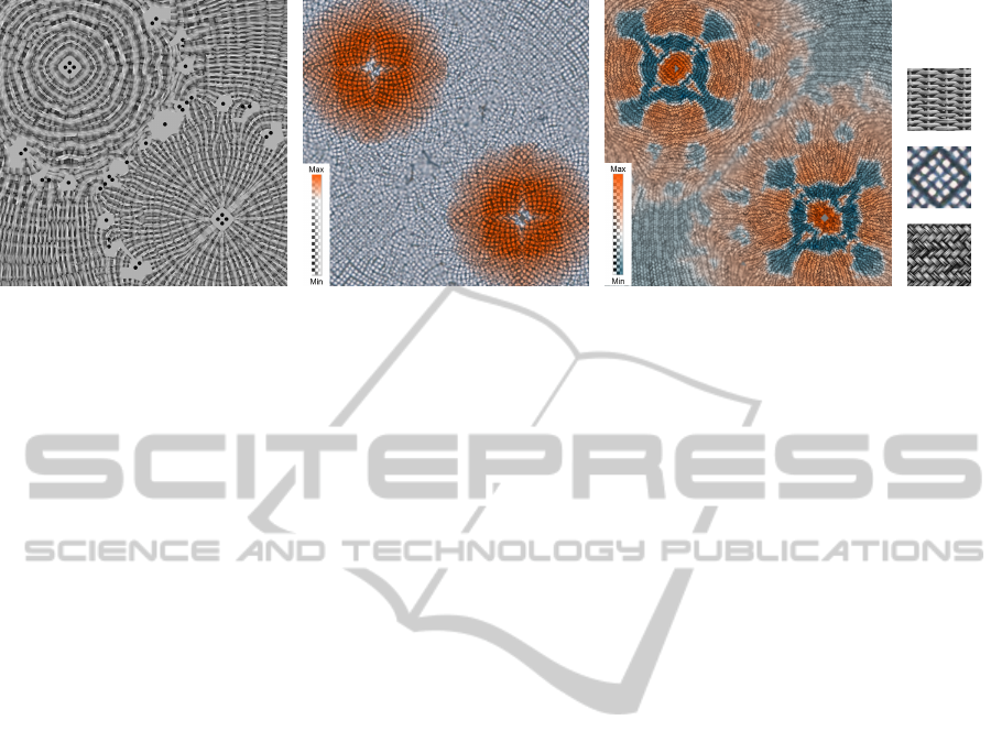
(a) (b) (c) (d)
Figure 7: Data set: Two-point load. Comparison of rendering with different input textures. (a) Bidirectional weave input
pattern, the frequency is adjusted to the mapped eigenvalues. (b) Rendering of the directions of maximal shear. Regions of
high maximal shear stress are emphasized in red. Regions of low maximal shear are blurred. (c) Knitting pattern emphasizing
major eigenvector directions from far, in detail directions of maximal shear are perceivable. Color coding is applied according
to the relative shear stress. (d) Shows from top to bottom the used sample patterns in Figures (a-c).
A similar visualization approach is applied to the
one-point load in Figure 6(a). Here the color cod-
ing corresponds directly to the mapped eigenvalues
(Eq. 2). Anisotropic regions are still discernible as
the superposition generates mixed colors for strongly
differing eigenvalues. Specific regions can be high-
lighted additionally by applying the post-processing
step: in Figure 6(b) regions with low relative shear
are blurred. The focus of the user is directed to
anisotropic regions, where eigenvalues exhibit a large
difference.
The versatility and power of textures is demon-
strated in Figure 7. For texture samples with inherent
natural variance discontinuities due to hanging nodes
in the original segmentation are less prominent. In
Figure 7(a) a weave input pattern is employed to vi-
sualize the eigenvector directions. Due to the bidi-
rectional nature of the weave pattern both eigenvector
fields are visualized at once. In Figure 7(b) the user
can switch to investigate directions of maximum shear
of the underlying field. Here a texture is used with
line structures illustrating the bisectors of the eigen-
vector directions. Additionally regions of high max-
imal shear stress (Eq. 1) are emphasized by selective
color mapping. The third example, Figure 7(c), gener-
ates a texture that resembles a knitted piece of fabric.
7 CONCLUSIONS
We have combined the accuracy of topological meth-
ods for two dimensional symmetric tensor fields with
the support of more intuitive visualizations. Our ap-
proach uses the strength of textures for continuous vi-
sualizations and allows to gain insight into detailed
information at discrete locations by placing glyphs.
A specific topology-based segmentation framework
(Auer et al., 2011) is used to employ these tech-
niques. The cells of this segmentation provide a con-
sistent parametrization for the texture mapping and
the bounding tensorlines correctly predetermine the
the eigenvector directions within. A multitude of pos-
sible textures can be implemented illustrating a har-
monious continuous view on the various tensor prop-
erties. A selection of textures is presented that encode
directional features; simple stripe textures but also
textures with higher inherent variance, that support a
smooth appearance over uneven transitions (hanging
nodes). We believe the latter textures can also be used
for other approaches that aim the mapping of direc-
tional textures region- oder cell-wise without appar-
ent distorted behavior at the boundaries.
Physical properties of the tensor field like compres-
sion or expansion are reflected in the texture fre-
quency. Selective color mapping and post process-
ing are applied to direct the users attention to scalar
features of interest. Certainly, there remains a large
potential to optimally assist the perceptional habits of
a user. We also presented this work as flexible basis
for further advancement.
ACKNOWLEDGEMENTS
This work was funded by the German Research
Foundation (DFG) through a Junior Research Group
Leader award (Emmy Noether Program).
IVAPP 2012 - International Conference on Information Visualization Theory and Applications
676

REFERENCES
Auer, C., Sreevalsan-Nair, J., Zobel, V., and Hotz, I. (to ap-
pear 2011). 2D Tensor Field Segmentation. In Scien-
tific Visualization: Interactions, Features, Metaphors,
volume 2 of Dagstuhl Follow-Ups.
Cabral, B. and Leedom, L. C. (1993). Imaging Vector Fields
Using Line Integral Convolution. In Proc. of the 20th
annual conference on Computer graphics and inter-
active techniques, pages 263–270.
Delmarcelle, T. (1994). The Visualization of Second-order
Tensor Fields . PhD thesis, Stanford University.
Delmarcelle, T. and Hesselink, L. (1993). Visualization of
Second Order Tensor Fields and Matrix Data. IEEE
Computer Graphics & Applications, pages 25–33.
Dick, C., Georgii, J., Burgkart, R., and Westermann, R.
(2009). Stress Tensor Field Visualization for Implant
Planning in Orthopedics. IEEE Transactions on Visu-
alization and Computer Graphics, 15(6):1399–1406.
Feng, L., Hotz, I., Hamann, B., and Joy, K. (2008).
Anisotropic Noise Samples. IEEE Transactions on Vi-
sualization and Computer Graphics, 14(2):342–354.
Hashash, Y. M. A., Yao, J. I.-C., and Wotring, D. C.
(2003). Glyph and Hyperstreamline Representation
of Stress and Strain Tensors and Material Constitutive
Response. Int. Journal for Numerical and Analytical
Methods in Geomechanics, 27(7):603–626.
Hesselink, L., Levy, Y., and Lavin, Y. (1997). The Topology
of Symmetric, Second-Order 3D Tensor Fields. IEEE
Transactions on Visualization and Computer Graph-
ics, 3(1):1–11.
Hlawitschka, M., Scheuermann, G., and Hamann, B.
(2007). Interactive Glyph Placement for Tensor
Fields. In ISVC (1), pages 331–340.
Hotz, I., Feng, L., Hagen, H., Hamann, B., Jeremic, B., and
Joy, K. (2004). Physically Based Methods for Tensor
Field Visualization. In Proc. of IEEE Visualization
(Vis’04), pages 123–130.
Hummel, M., Garth, C., Hamann, B., Hagen, H., and Joy,
K. I. (2010). IRIS: Illustrative Rendering for Inte-
gral Surfaces. IEEE Transactions on Visualization and
Computer Graphics, 16:1319–1328.
Kindlmann, G. and Westin, C.-F. (2006). Diffusion Ten-
sor Visualization with Glyph Packing. IEEE Trans-
actions on Visualization and Computer Graphics,
12(5):1329–1336.
Kratz, A., Kettlitz, N., and Hotz, I. (2011). Particle-Based
Anisotropic Sampling for Two-Dimensional Tensor
Field Visualization. In Vision Modeling and Visual-
ization (VMV’11), pages 145–152.
Lavin, Y., Batra, R., Hesselink, L., and Levy, Y. (1997). The
Topology of Symmetric Tensor Fields. AIAA Compu-
tational Fluid Dynamics Conference,, page 2084.
Rustamov, R. M., Lipman, Y., and Funkhouser, T. (2009).
Interior Distance Using Barycentric Coordinates. In
Proc. of the Symposium on Geometry Processing
(SGP ’09), pages 1279–1288.
Schultz, T. and Kindlmann, G. (2010). Superquadric
Glyphs for Symmetric Second-Order Tensors. IEEE
Transactions on Visualization and Computer Graph-
ics, 16:1595–1604.
Sreevalsan-Nair, J., Auer, C., Hamann, B., and Hotz, I.
(2010). Eigenvector-based Interpolation and Segmen-
tation of 2D Tensor Fields. In Topological Methods
in Visualization. Theory, Algorithms, and Applications
(TopoInVis 2009).
Tricoche, X., Kindlmann, G. L., and Westin, C.-F. (2008).
Invariant Crease Lines for Topological and Structural
Analysis of Tensor Fields. IEEE Transactions on Visu-
alization and Computer Graphics, 14(6):1627–1634.
Tricoche, X., Scheuermann, G., Hagen, H., and Clauss, S.
(2001). Vector and Tensor Field Topology Simplifica-
tion on Irregular Grids. In Proceedings of the Sympo-
sium on Data Visualization (VisSym ’01), pages 107–
116.
Zheng, X. and Pang, A. (2003). HyperLIC. In Proc. of
IEEE Visualization (Vis’03), pages 249–256.
Zheng, X. and Pang, A. (2004). Topological Lines in 3D
Tensor Fields. In Proc. of IEEE Visualization (Vis’04).
GLYPH- AND TEXTURE-BASED VISUALIZATION OF SEGMENTED TENSOR FIELDS
677
