
SURFACE-BASED SEGMENTATION OF 3D POINT CLOUD DATA
IN THE VECTOR FIELD REPRESENTATION
Van Tung Nguyen and Denis Laurendeau
Computer Vision and System Laboratory, Laval University, Quebec City, QC, Canada
Keywords:
3D Segmentation, Surface Modeling, Volumetric Representation.
Abstract:
In this paper, we propose an approach for 3D segmentation of point cloud data based on the vector field
representation. A volumetric surface representation named the vector field is first computed for the input
point cloud. The data description in a voxel of the vector field is then classified into eight surface types
by computing the sign of curvatures for the closest point of the voxel on the surface. A region-growing
sheme based on bivariate fuctions fitting is finally applied to the closest points of these voxels for refining the
segmented regions. This surface-based approach is entirely designed in the vector field surface representation
and the advantages of using the vector field are discussed. Experiments demonstrate the peformance of the
method.
1 INTRODUCTION
Segmentation is an essential step that can be found in
many research areas in computer vision such as shape
retrieval, compression, registration, and object recog-
nition. Basically, 3D segmentation consists of seg-
menting the input data into a set of meaningful “geo-
metric” parts or regions in the scene. Due to the im-
portance of this step in 3D applications, many seg-
mentation techniques have been developed that can
roughly be classified in two main categories: edge-
based and surface-based techniques (Hoover et al.,
1996)(Besl and Jain, 1988). In general, the former use
edge detection to create region boundaries (Hoover
et al., 1996)(Zhang et al., 2008) while the latter use
analytic surface description to divide the image into
disjoint regions (Besl and Jain, 1988)(Besl and Jain,
1986)(Zheng et al., 2008)(Gelfand and Guibas, 2004).
In this paper, a surface-based segmentation tech-
nique for 3D point cloud data is presented. Our goal is
to propose a segmentation technique that always min-
imizes computational load at every steps in the algo-
rithm by using the vector field representation. The
vector field representation, introduced in the next sec-
tions helps to reduce the complexity of neighbour-
hood operations often required by surface-based seg-
mentation approaches. Our approach first computes
the vector field from the input data. Then points be-
longing to regions with similiar geometric properties
are classified into eight types of surface geometry ba-
sed on local curvature properties computed from the
vector field representation. A region growing scheme
based on the fitting of low- order bivariate functions
is then performed on the initial set of regions to refine
the segmentation.
The paper is organized as follows. First the vector
field framework and curvature estimation approach
are presented in Section 2. Section 3 presents the
proposed segmentation technique including the ini-
tial region finding process and the refinement process.
Next, experiments show the results demonstrating the
performance of the method. Section 5 discusses the
results and proposes future work.
2 CURVATURE ESTIMATION IN
THE VECTOR FIELD
REPRESENTATION
We first introduce the terminology relevent to the vec-
tor field surface representation computed for point-
set data and then extend the framework to introduce
a computational method for curvature estimation on
the vector field.
2.1 The Vector Field Representation
In 3D modeling, representation of 3D data is a very
important issue since it has an impact on the compu-
157
Tung Nguyen V. and Laurendeau D..
SURFACE-BASED SEGMENTATION OF 3D POINT CLOUD DATA IN THE VECTOR FIELD REPRESENTATION.
DOI: 10.5220/0003857601570162
In Proceedings of the International Conference on Computer Graphics Theory and Applications (GRAPP-2012), pages 157-162
ISBN: 978-989-8565-02-0
Copyright
c
2012 SCITEPRESS (Science and Technology Publications, Lda.)

tational complexity of the segmentation steps. Three
main 3D representation methods- mesh, volumetric
grids and polynomial representations- have been pro-
posed in the literature(Zheng et al., 2008)(Tubic et al.,
2002)(Zhang et al., 2008). Each type of representa-
tion has its advantages and disadvantages. In addition,
the chosen representation of the input data affects the
data segmentation and surface modelling steps sig-
nificantly. In 2002, Tubic et al. (Tubic et al., 2002)
proposed a new implicit surface representation called
the “vector field”. The vector field framework has
demonstrated its capacity of unifying all steps of in-
terative 3D modeling (registration, integration, mod-
elling and visualization) in one type of data represen-
tation with linear computational complexity (Tubic
et al., 2004).
voxel
vector toward the
normal to the
closest point on
the surface
envelope
Point set
and surface
Figure 1: Vector field representation.
In essence, the vector field is a volumetric repre-
sentation where each voxel encodes the vector point-
ing from the voxel center to the closest point on the
surface to be modeled. Suppose that point cloud data
is available, the vector field is built by updating the
covariance matrix C at each voxel located nearby data
point p
i
inside an envelope of size ε (Tubic et al.,
2002):
C =
1
N
N
∑
i=1
(p
i
−
˜
p)(p
i
−
˜
p)
T
=
1
N
N
∑
i=1
p
i
p
T
i
−p
i
p
T
i
(1)
where
˜
p =
1
N
∑
N
i=1
p
i
and N the number of points that
have already participated in the voxel updates.
The eigenvector associated with the smallest
eigenvalue of the covariance matrix represents the
normal vector N to the tangent plane at the closest
point, then the direction of the vector field F(v) at the
voxel v is computed as:
F(v) = N
h
N,
˜
p − v
i
(2)
where
h
.
i
is the scalar product.
Figure 1 shows a 2D view of a vector field repre-
sentation, all the voxels within the envelope (bounded
by the dashed line) are updated with the information
of the point set on the surface (in black). The envelope
is used to determine the number of local voxels sur-
rounding the surface in which the vector field is up-
dated for each incoming data point. The envelope size
and voxel size is always a trade-off. A large envelope
size or a small voxel size results in a dense vector field
and increases the accuracy at the reconstruction step
but increases computational complexity and memory
requirements for storing the vector field. Practically,
the envelope size is chosen twice the voxel size. As an
expansion to this basic definition of the vector field,
we define two types of voxels: active voxels and sur-
face voxels. An active voxel is one that contains vec-
tor field information pointing toward the closest point
on the surface (the voxels within the envelope in Fig-
ure 1). A surface voxel is an active voxel crossed by
the surface (for the point cloud data, that is an active
voxel contains the points on the surface). This con-
dition can be easily checked by finding whether or
not the closest point encoded by a surface voxel is lo-
cated inside this voxel (the surface voxels are colored
in red in the example on Figure 1). Given the exten-
sion, it will be shown next that only the curvatures at
the closest points of the surface voxels are computed
using the closest points of neighbouring active voxels
and only the closest points of the surface voxels con-
tribute to the estimation of the fitting functions in the
segmentation process.
2.2 Curvature Estimation
Based on the vector field framework described above,
we propose a scheme for estimating curvatures at the
closest point of each surface voxels (Nguyen and Lau-
rendeau, 2011). To do this, at a surface voxel, we de-
tect the closest point on the surface by the encoded
vector field value then, the other closest points of
neighbouring active voxels are used to estimate the
curvature at this point. This approach based on the
vector field departs significantly from approaches that
compute curvature directly from the point cloud data.
As shown in Figure 2, to collect neighbouring points
of a given point p for estimating the curvatures, all
the points in the circle of radius r centered at p are
searched. In Figure 2.a, all points in the green re-
gion are obtained by the search. This search is hard to
achieve in a point cloud because nearest neighbours
must be found. However, in the vector field represen-
tation, this search becomes an easy task by detecting
the neighbouring voxels, then collecting the closest
points of these active voxel that contribute to curva-
ture estimation because nearest information is stored
directly in the field. In Figure 2.c, all neighbour vox-
els of a given voxel containing p are detected and
highlighted by light green colour, but only active vox-
GRAPP 2012 - International Conference on Computer Graphics Theory and Applications
158

els are considered for the curvature estimation (light
green voxel in Figure 2.d). Changing the size of ra-
dius r to have more neighboring points in the search
is approximated by adding more layers of neighbour-
ing voxels in the curvature computation with the vec-
tor field.(Figure 2.e and Figure 2.f show example of
two layers for detecting the neighbour voxels). Prac-
tically, the size of r or extention of more layers search
in the vector field for collecting more neighboring
points is chosen suitable with the geometry of the
scene.
p
r
(a) (b)
(c) (d)
(e) (f)
Figure 2: Illustration of neighbouring voxels detection for
cuvature computation using the vector field. (a) shows the
search with point cloud directly, (b) is the encoded vec-
tor field, (c) shows all the neighbouring voxels detected in
green for the center voxel in red and (d) shows the neigh-
bouring active voxels taken into account for curvature es-
timation, (e),(f) shows an example of the two voxel layers
search.
After detecting the neighbours to be considered
for curvature estimation, the method described by
Chen and Schmitt (1992) is used for estimating the
curvatures at a point using normal vectors and their
neighbouring points (Chen and Schmitt, 1992)(Dong,
2005). In our case, the normal vectors at the closest
points are implicitly encoded in the vector field (as
shown in Figure 1) since the field contains the direc-
tion of the closest point at the surface and Chen and
Schmitt’s method is exploited as follows.
Let us assume that a point p has m neighbours.
The main idea in this method is to choose a suitable
coordinate system (
ˆ
e
1
,
ˆ
e
2
) for a group of unit length
tangent vectors t on the local tangent plane at point p.
The normal vectors at that point and its neigbours are
used to estimate the normal curvatures k
n
(t
i
) along
the tangent direction t
i
on the local tangent plane at p
as follows (Chen and Schmitt, 1992)(Dong, 2005):
k
n
(t
i
) = −
h
p
i
− p,N
i
− N
i
h
p
i
− p,p
i
− p
i
(3)
t
i
=
(p
i
− p) −
h
p
i
− p,N
i
N
k
(p
i
− p) −
h
p
i
− p,N
i
N
k
(i=1,2..m) (4)
where
k
.
k
is the Euclidean norm of a vector and N
i
and N are normal vectors at p
i
and p. Suppose that
k
n
(t
id
) is the maximum of the normal curvatures cor-
responding to the tangent direction t
id
. Then, the spe-
cial coordinate system (
ˆ
e
1
,
ˆ
e
2
) on the tangent plane at
p can be chosen as follows:
ˆ
e
1
= t
id
,
ˆ
e
2
=
ˆ
e
1
× N
k
ˆ
e
1
× N
k
(5)
From this, a set of m equations is obtained according
to Chen and Schmitt’s method:
k
n
(t
i
) = a cos
2
(θ
i
)+bcos(θ
i
)sin(θ
i
)+csin
2
(θ
i
) (6)
where θ
i
is the angle between t
i
and
ˆ
e
1
(i=1,2..m).
A least-squares method is used for solving the set of
equations for the coefficients a, b and c. This leads to
the Gaussian curvature(K), mean curvature (H) and
two principal curvatures k
1,2
as follows:
K = ac −b
2
/4, H = (a + c)/2, and
k
1,2
= H ±
p
H
2
− K (7)
3 SEGMENTATION IN THE
VECTOR FIELD
REPRESENTATION
As presented by Besl in 1988, using the sign of the
Gaussian and mean curvatures at points on a smooth
surface, the surface can be decomposed into a union
of simple surface patches that are approximated by bi-
variate polynomials with order lower than four (Besl
and Jain, 1986). In this section, we borrow Besl’s ap-
proach for segmenting surfaces based on the sign of
the curvatures and then use a region growing fitting
process to refine the initial segmentation. With some
assumptions, Besl’s approach is implemented in the
vector field representation.
SURFACE-BASED SEGMENTATION OF 3D POINT CLOUD DATA IN THE VECTOR FIELD REPRESENTATION
159

3.1 Initial Segmentation with the Sign
of Curvatures
In section 2.2 we presented a method for estimating
the curvatures at the closest points of the surface vox-
els in the vector field representation. Based on the
fact that surface characteristics are almost identical on
a small region surrounding a point, we use the clos-
est points as “prominent points” that characterize sur-
rounding regions occupied by the surface voxels. This
means that, based on the surface shape determined by
the curvature signs at a “prominent point” on the sur-
face, the region occupied by the corresponding sur-
face voxel belongs to the same surface type. Figure
3 shows the eight fundamental surface shapes possi-
ble based on the Gaussian and mean curvatures at a
prominent point (Besl and Jain, 1986).
Peak Surface
H<0, K>0
Flat Surface
H=0, K=0
Pit Surface
H>0, K>0
Ridge Surface
H<0, K=0
Minimal Surface
H=0, K<0
Saddle Ridge
H<0, K<0
Valley Surface
H>0, K=0
Saddle Valley
H>0, K<0
Figure 3: Eight fundamental surface types (Besl and Jain,
1986).
Therefore, in this initial segmentation step, the
surface is decomposed into small disjoint regions be-
longing to one of eight possible surface types by la-
beling surface types of “prominent point”. Figure 4
shows an example of how this initial segmentation is
obtained. A surface (Figure 4.a) is encoded by the
vector field as shown in Figure 4.b. The surface voxels
with different colours express different shape types
(illustrated in Figure 3) of the “prominent point” of
these voxel respectively. Then the regions occupied
by these surface voxels have the same shape type (Fig-
ure 4.c). Figure 4.d shows the surface classified by
regions with different shape type expressed by differ-
ent colours. Section 4 will shows some typical results
obtained by the first segmentation step.
3.2 Refined Segmentation with Region
Growing
The region growing scheme is responsible for merg-
ing the coarse segmented regions obtained in the
above initial step to create larger surface patches. In
fact, it is the process of spreading out initial patches
from a seed region. As presented by Besl(Besl and
(a) (b)
(c) (d)
Figure 4: Illustration of ideal results obtained from the ini-
tial segmentation. (a) is an example of input surface; (b) is
the vector field with the surface types stored in the surface
voxels in different colours; (c) regions crossed by the voxels
have the same surface types; (d) regions in different colour
are obtained by the initial segmentation.
Jain, 1988), the curvature-sign primitives classified by
the initial step presented above can be approximated
well by a bivariate function with order lower than four
as illustrated next.
Suppose that a smooth surface is a twice-
differentiable function z=f(x,y). The form of the fit-
ting function can be written as follows:
ˆ
f (m,a;x,y) =
∑
i+ j≤m
a
i j
x
i
y
j
= a
00
+ a
10
x + a
01
y + a
11
xy + a
20
x
2
+a
02
y
2
+ a
21
x
2
y + a
12
xy
2
+ a
30
y
3
+a
03
y
3
+ a
31
x
3
y + a
22
x
2
y
2
+a
13
xy
3
+ a
40
x
4
+ a
04
y
4
(8)
Where, m≤4 is the order of the function and the
function can be expressed for a planar, biquadratic,
bicubic and biquartic surface with the length of the
coefficient vector a corresponding to 3, 6, 10 and
15. The surface fitting function minimizes the least-
squares error metric
ε =
1
N
N
∑
i=1
(
ˆ
f (m,a;x,y) − f (x,y))
2
(9)
Where N is the number of points contributing to the
estimation of the fitting function. The region-growing
scheme based on this fitting of functions in the vector
field representation is as follows.
First, the surface shape types of the prominent
points set (the closest points of surface voxels) ob-
tained at the initial step are stored at the correspond-
ing surface voxels and coordinates of the prominent
GRAPP 2012 - International Conference on Computer Graphics Theory and Applications
160

points are extracted and stored in a list of set of promi-
nent points for the next processing step as shown in
Figure 5 (different colours of voxels are used for dif-
ferent shape types). This configuration helps to avoid
checking all voxels to find a surface voxel as a start-
ing point. Instead of checking all voxels to detect a
surface voxels, starting from a point in this list allows
to detect which surface voxel the point falls into.
.
.
.
List of
examined
prominent
points
A point in the
list and its
corresponding
voxel
Figure 5: Explanation of the configuration for growing fit-
ting in the vector field.
Two key elements of a region growing process are
finding a starting seed point and defining a stopping
criterion. For finding a good seed region, we start
with a prominent point in the list to detect to which
surface voxel it belongs to. Based on the detected
surface voxel, we consider its neighbouring surface
voxels to check whether or not these voxels are la-
beled with the same surface type. If it is the case, then
we have a “trustable” seed region to start the region
growing process with the closest points corresponding
to the surface voxels. The expansion process to find
neighboring closest points for the surface fitting pro-
cedure becomes easy by detecting neighboring sur-
face voxels (the same as shown in the Figure 2). When
a surface voxel is considered and its prominent point
has successfully contributed to the surface fitting esti-
mation, it is assigned the label ’visited’ to avoid mul-
tiple scan for the corresponding closest point. For a
seed region, the stopping criterion is when the error
metric in the equation (9) is greater than a threshold
while the highest order of the bivariate function has
been reached (m=4). The idea of variable-order poly-
nomial fitting proposed by Besl is used: each time a
seed region is chosen, we first try to fit with a plane to
the region (length of the coefficent a is 3). If it is not
suitable (error metric is larger than the threshold), we
move to higher order surfaces (biquadratic, bicubic,
and biquartic surface, where a is 6, 10 and 15 respec-
tively). The overall decision to stop the fitting process
of the region growing on the surface is to check if all
selected prominent points from the list fall into a ’vis-
ited’ surface voxel. This means that all regions on the
surface have been visited.
4 EXPERIMENTAL RESULTS
For validation, the proposed method is applied to
some popular testing objects. The envelope size of the
vector field is always chosen as twice of voxel size,
and the size of voxel is chosen depending on resolu-
tion of object. To get the sign of Gaussian and Mean
curvatures, curvature is set to zero when it is smaller
than 0.4% of the maximum absolute value of curva-
ture. The threshold for the error in the fitting process
is set to 0.5 of the voxel size.
For curvature estimation using the vector field,
Figure 6 shows the colormap of Gaussian and Mean
curvatures estimated for the budda model. Colour
change corresponds to a change in minimum to max-
imum estimated value of the curvatures. The resolu-
tion of the budda model is good, so the estimated cur-
vature values are reliable given by the smooth change
in colours in the figure. With this model, the voxel
size is set 0.001.
(a) Gaussian curvature. (b) Mean curvature.
Figure 6: Colormap of estimated curvatures for the budda
model.
(a) (b)
(c)
Figure 7: Surface segmentation on a simple object. (a) view
of the surface of the surface object, (b) initial segmentation,
(c) refined segmentation.
SURFACE-BASED SEGMENTATION OF 3D POINT CLOUD DATA IN THE VECTOR FIELD REPRESENTATION
161
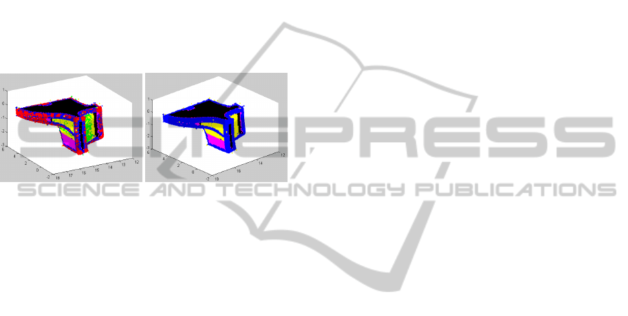
Figure 7 shows the segmentation of a simple ob-
ject. Figure 7.b shows the result of the initial segmen-
tation. Surface regions of different surface types are
shown in different colours. The initial step includes
some fragmented regions caused by wrong estimated
curvature sign. Figure 7.c shows the improvement of
the result after applying the refinement segmentation
process. Because the vector field implicitly contains
reconstruction information, the algorithm for the re-
finement process is designed to refine the shape type
of the surface to get segmented regions separated by
shape boundaries. The voxel size is set 0.18 for this
object.
(a) (b)
Figure 8: Surface segmentation on an object. (a) initial seg-
mentation, (b) refined segmentation.
Figure 8.a shows the prominent points (closest
points on the surface of surface voxels) reconstructed
for another object after the initial segmentation step.
Different colours express different surface types of
the points. Figure 8.b shows the improved result com-
posed of reliable regions after the refinement process.
Voxel size is set 0.065 for this object. The algorithm
is currently being improved to reduce the thickness of
boundaries on these objects.
5 CONCLUSIONS
A new mechanism for 3D segmentation was intro-
duced for point-set data in the vector field surface
representation. An initial segmentation process is
first proposed by segmenting the surface into disjoint
regions labeled by eight fundamental surface types.
Then the segmented regions are improved by a region
growing process based on bivariate function fitting.
Designing the segmentation mechanism in the vec-
tor field allows to keep computation simple and avoid
complex nearest neightbour search for curvature esti-
mation and spreading out in the region growing pro-
cess. Several directions are possible for future work.
For instance an adaptive scaling in computing local
features such as curvatures could help to avoid seed
region to be too fragmented. Robustness to noise will
also be investigated.
REFERENCES
Besl, P. J. and Jain, R. C. (1986). Invariant surface char-
acteristics for 3D object recognition in range images.
Computer Vision, Graphics, and Image Processing,
33:3380. ACM ID: 7056.
Besl, P. J. and Jain, R. C. (1988). Segmentation
through variable-order surface fitting. IEEE Transac-
tions on Pattern Analysis and Machine Intelligence,
10(2):167–192.
Chen, X. and Schmitt, F. (1992). Intrinsic surface prop-
erties from surface triangulation. In Proceedings of
the Second European Conference on Computer Vision,
ECCV ’92, pages 739–743, London, UK. Springer-
Verlag.
Dong, C. Wang, G. (2005). Curvatures estimation
on triangular mesh. Journal of Zhejiang Uni-
versity (SCIENCE), Journal of Zhejiang University
(SCIENCE):128–136.
Gelfand, N. and Guibas, L. J. (2004). Shape segmentation
using local slippage analysis. In Proceedings of the
2004 Eurographics/ACM SIGGRAPH symposium on
Geometry processing, SGP ’04, page 214223, New
York, NY, USA. ACM.
Hoover, A., Jean-baptiste, G., Jiang, X., Flynn, P. J., Bunke,
H., Goldgof, D., Bowyer, K., Eggert, D., Fitzgibbon,
A., and Fisher, R. (1996). An experimental compar-
ison of range image segmentation algorithms. IEEE
Transactions on Pattern Analysis and Machine Intel-
ligence.
Nguyen, V. and Laurendeau, D. (2011). A global regis-
tration method based on the vector field representa-
tion. In 2011 Canadian Conference on Computer and
Robot Vision (CRV), pages 132–139. IEEE.
Tubic, D., Hebert, P., Deschenes, J., and Laurendeau, D.
(2004). A unified representation for interactive 3D
modeling. In 3D Data Processing, Visualization and
Transmission, 2004. 3DPVT 2004. Proceedings. 2nd
International Symposium on, page 175182.
Tubic, D., Hebert, P., and Laurendeau, D. (2002). A volu-
metric approach for the registration and integration of
range images: towards interactive modeling systems.
In Pattern Recognition, 2002. Proceedings. 16th In-
ternational Conference on, volume 3, pages 283–286
vol.3.
Zhang, X., Li, G., Xiong, Y., and He, F. (2008). 3D
mesh segmentation using mean-shifted curvature. In
Proceedings of the 5th international conference on
Advances in geometric modeling and processing,
GMP’08, page 465474, Berlin, Heidelberg. Springer-
Verlag.
Zheng, B., Takamatsu, J., and Ikeuchi, K. (2008). 3D model
segmentation and representation with implicit polyno-
mials. IEICE - Trans. Inf. Syst., E91-D(4):11491158.
GRAPP 2012 - International Conference on Computer Graphics Theory and Applications
162
