
INTRODUCTION TO MULTICRITERIA TECHNIQUES
Jorge Azevedo Santos
1
and Elsa Rosário Negas
2
1
Research Centre in Mathematics and Applications (CIMA), University of Évora, Évora, Portugal
2
Centre for Research and Development in Territory, Architecture and Design (CITAD),
Lusíada University of Lisbon, Lisbon, Portugal
Keywords: Decision theory, Multiobjective, Multicriteria trident, Electre, Data envelopment analysis.
Abstract: The systematic analysis and decision making in companies, particularly in an environment of risk, are now a
major challenge, namely the complexity of each problem. Multicriteria techniques are applied a long time
ago and had an important development and expanded its application areas. The simple decisions, which are
considered routine, given the frequency they repeat themselves tend now to be reviewed and reanalyzed in
order to be efficient. Sort a decision as efficient as we rank a decision when compared with other decisions
in which the chosen factors have worse performance, or deciding factors, for example, the ratio between
consumption and production is less attractive.
1 THE COLLECTION
OF INFORMATION
AND FORMULATION
OF THE PROBLEM
By analyzing a situation it is necessary to know the
surrounding primarily internal and external
environment. It is necessary to collect information
about the company, its employees, its suppliers, its
customers and to the legislation that regulates it,
which is characterized by internal environment.
Collect information about competitors, industry
sector, European law in the case of application of
quotas, which is characterized by the external
environment.
Currently Operational Research offers a large set
of theories, methods and models that allow the
decision maker to reduce the degree of uncertainty
in decision making as it can rely on models already
tested and widely applied in different sectors.
The complexity of decisions are now often very
large part of every decision and serves as a "lever"
for the other decisions which influence and are
influenced and, moreover, often increasing the
complexity of using same resources, which involves
choices regarding the allocation of human or
material resources.
Reflecting the rapid evolution of markets but
also the enormous dependence of each sector of the
global economy, decisions are made based on
deterministic models that do not increase the
uncertainty of each decision, linked to other
decisions that greatly increases the randomness.
The decision maker can minimize risk by
collecting and "working" all available information
concerning the system where it operates, the
company he represents, to competitors, it aims to
meet customers, regulators, among others.
Among the various paradigms presented by
(Valadares Tavares et al. 1996) we emphasize the
effectiveness of: while not ignoring the multiple
sources of uncertainty and randomness, it is believed
in the ability to establish effective systems, ie
systems that achieve goals with predefined levels of
safety or reliability very high.
One should emphasize the difference between
decision making in nonprofit organizations, private
enterprises and public enterprises which is justified
by the difference in the Mission.
The set of steps are: comprehensive listing of all
resources (human, financial and technical); listing of
all feasible alternatives, identify the criteria that will
influence and ultimately quantify each alternative /
criterion.
2 PROBLEM FORMULATION
After the development of all the steps mentioned
490
Santos J. and Rosário Negas E..
INTRODUCTION TO MULTICRITERIA TECHNIQUES .
DOI: 10.5220/0003857804900494
In Proceedings of the 1st International Conference on Operations Research and Enterprise Systems (ICORES-2012), pages 490-494
ISBN: 978-989-8425-97-3
Copyright
c
2012 SCITEPRESS (Science and Technology Publications, Lda.)
above the decision maker is faced with a set of
alternatives which will select one based on clearly
defined criteria.
A scale is assigned for each criterion which is
defined by the amplitude, ie, a maximum value,
minimum value and even the definition whether this
criterion should be maximized or minimized.
If each criterion has a range quite different,
which influences the results it does not raise any
issue because they simply become more consistent.
Set of Alternatives - A1; A2; A3;…; Ai
In order not to increase the complexity in solving
the problem but to enter into account all factors
relevant to the decision. Each criterion is to be
analyzed individually or as a result of the analysis
criteria of any other criteria, which implies a
decrease in complexity.
According to the scale given to each criterion,
each alternative is quantified for each criterion and
Xij represents the quantification assigned to
alternative i according to the criterion j.
Quantification Xij may correspond to a
numerical scale or a qualitative scale (attributes).
The subordination of criteria is when the
decision maker can define a relationship between the
relative importance of these values (Keeney 1988
and 1992). Each structure of this type characterizes
their own ethics (Valadares Tavares et. al., 1996) not
only the decision maker but the system where it is
inserted. Even before choosing and applying the
model one should identify all situations of
subordination and eliminate all these dominated
alternatives.
To evaluate a set of alternatives based on
different criteria there are several methods in this
paper we analyze:
• Compensating Methods;
• Non-Compensatory Models.
We will use software MacModel created in 2001
by José Coelho in IST (Instituto Superior Técnico)
to multicriteria problem solving which will consist
of the presentation of some outputs and especially
the results and sensitivity analysis.
3 COMPENSATORY MODELS
Why use the term compensatory? It comes from the
fact that an alternative may have certain criteria in a
quantifier worst since the other criteria can restore
the balance.
This is because this model aims at the integration
of different criteria which is easily achieved by
assigning each criterion a preference indicator, each
indicator varies between 0 and 1 and the sum of all
indicators is equal to unity. The indicator preferably
assigned to each criterion represents the weight of
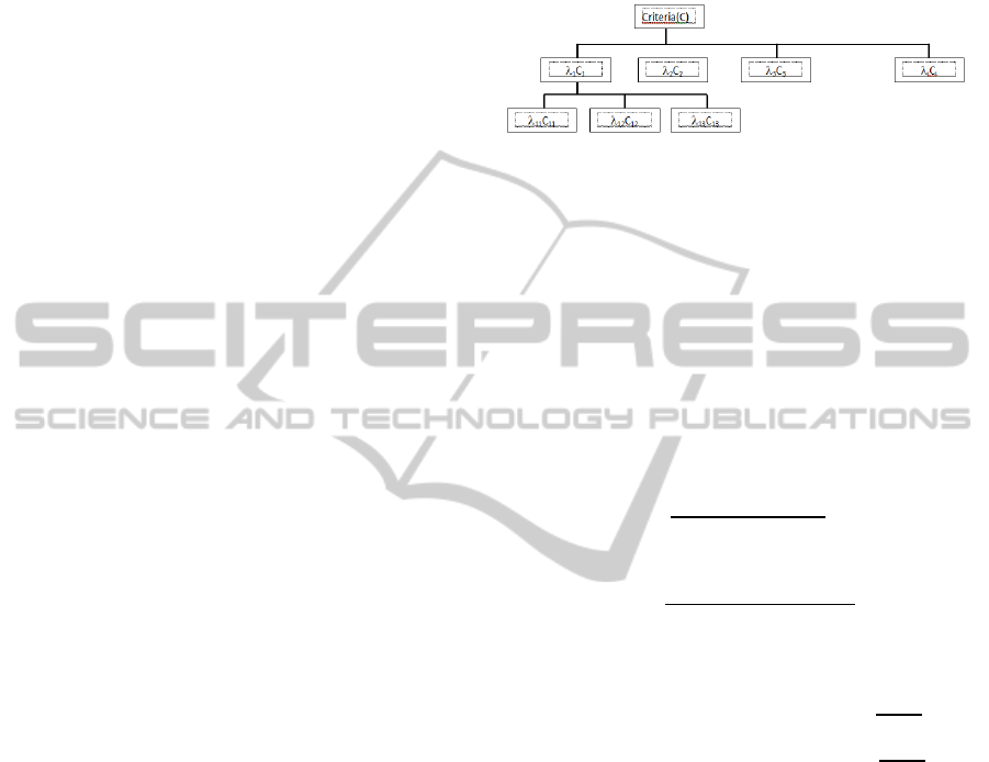
each criterion in the final decision. Representing a
tree in the same scheme previously presented:
Figure 1: Assigning weights to each criterion and each
sub-criterion.
∑
=1
Trade-off between criteria a and b is calculated
as follows: (Valadares Tavares et. al, 1996):
,
=
Often the criteria are not expressed on the same
scale, which in real terms is quite likely, therefore it
is necessary to standardize each scale applying the
following equations:
In the case of increasing preference
=
In the case of decreasing preference
x
=
max
X
−X
max
X
−min
X
Another possibility is to use the following formulas:
In case of increasing preference: x
=
In case of decreasing preference: x
=
Symbols µj and σj are the mean and standard
deviation respectively; min
i
(X
ij
) and max
i
(X
ij
) the
minimum and maximum for each criteria.
We perform the calculation for each alternative,
getting a weighted average. The weights are given
by the indicators of preference for each criterion and
the values considered are the measurements assigned
to each alternative (for each criteria),
=
∑
and
∑
=1
In the simple additive model the decision is
made by maximizing the values obtained.
In any decision-making process there are risks
and all methods present limitations, the limitations
of this model are presented in (Valadares Tavares et
al., 1996).
The best way to minimize risk is to reduce the
INTRODUCTION TO MULTICRITERIA TECHNIQUES
491

number of parameters considering only the most
relevant to decision making. And still must make the
application of the same scale for all criteria, or to
proceed to its standardization.
If there are two or three criteria they can be
represented graphically and make a sensitivity
analysis. This analysis is always important because
it allows us to identify the ranges for each λj in order
to remain the same solution; the stability of the
solution reduces uncertainty because it makes it so
relevant to the choice of the alternative to implement
the weighting given to each criterion or aggregation
of criteria.
Graphing is fairly simple if the number of
criteria we have is just two:
=
+
.
If there are three criteria begins with the
following transformation λ
3
=1-λ
1
+λ
2
then for each
alternative is identified
=
+
+(1−
−
)
then to represent each pair of
alternatives a line called the indifference which give
rise to different areas that will allow an analysis.
In this case the graphical representation ceases to
be simple but it will be easier to use the MacModel
software (Coelho, 2001).
The number of lines of indifference is given by
(
)
where m is the number of alternatives,
(Valadares Tavares et al., 1996).
4 NON-COMPENSATORY
MODELS
This method was developed by Bernard Roy in 1968
which to identify relationships of dominance
between two alternatives.
The comparison between alternatives is made for
the values j (all criteria) and results in a clash
between any two alternatives can be observed two
situations:
• condition of agreement, defined by the average
order of preference;
• condition of disagreement, a sense of "veto" the
decision maker can use when the average direction
of the disagreement is very strong in one criterion.
They also defined weights for different criteria.
The sum of the weights is unity.
The notion of integration remains of criteria, i.e.
a criterion can result from the integration of sub-
criteria, as in the previous process and weights are
also assigned to the sub criteria. But the analysis is
done using binary comparisons.
We use a relational system of preferences by
comparing the two alternatives.
Considering a practical application to three
criteria we will calculate binary comparisons between
any two alternatives thus obtaining R1, R2, R3.
When comparing the two alternatives we can
conclude that there is: indifference, equivalence or
dominance.
This method is applied on one hand to the
average order of preference and on the other to a
sense of veto in the case of the average direction of
disagreement to be very strong.
Note that this method can be applied even if the
quantifiers are attributes, xij is a qualitative variable.
When comparing two alternatives by applying
the condition of agreement it is necessary to
establish a value α (0 ≤ "α" ≤ 1) representing the
minimum amount required to be accepted that a
prevails over b:
=
∑
λ
:
≥
≥
α
The decision maker may also evaluate the
disagreement between two alternatives, calculating
the difference for each quantifier of the two
alternatives under study.
We will get j results in a problem with j criteria.
If the objective is to maximize, the greater of the
calculated values will be chosen. Getting just the
disagreement between any two alternatives, β
defines the maximum permissible level of
disagreement:
=max
−
≤
β
When the quantifiers are qualitative a
correspondence should be performed to a scale so
that the agreement can be calculated Similarly in the
case of disagreement the decision maker must decide
how many levels are considered severe enough to
apply the "veto". For example if the match is made
with mediocre, poor, fair, good and very good
condition and the disagreement is over 2 levels when
compared with the good will only be applied to the
mediocre.
The prevalence among alternatives is the more
difficult the higher the value assigned to α and lower
the value assigned to β.
The prevalence relation is not transitive. It is
likely that an alternative to prevail over another but
is dominated by another by analyzing three
alternatives.
In this case the decision process may not have
finished and be more advisable to collect
information, analyze more fully each of the
alternatives still under possible selection.
In all cases it will carry out sensitivity analysis
which is performed by changing the values of α and
ICORES 2012 - 1st International Conference on Operations Research and Enterprise Systems
492
β checking for intervals remain the same solutions
that will strengthen the choice of a particular
alternative.
5 APPLICATION TO A
PRACTICAL CASE
Consider six different locations to install a landfill.
All decision making is based on three criteria time,
cost and environmental impact. The latter is
considered as the aggregation of three sub criteria
pollution, aesthetic and Agricultural Land Unusable
(ALU).
The collection of information and different
measurements has been performed and is presented
in the following tables. Starting with the 3
rd
criteria
Environmental Impact, sub criteria are aggregated
using the following system of weights: 20%, 10%
and 70%, respectively, as shown below:
Table 1: Quantifiers linking each alternative to sub criteria
for Environmental Impact, values entered in MacModel.
Subcriteria Criteria
Pollution Aesthetic ALU Environmental
Locations
1 10 8 4 5.6
2 6 10 8 7.8
3 6 6 10 8.8
4 0 5 9 6.8
5 5 8 0 1.8
6 8 0 3 3.7
It is obvious that the aggregation weights for this
are debatable, and lend themselves to many other
possible choices. You can now submit all the values
for the three criteria and its value, the weights are
considered 10%, 25% and 65%, respectively,
Environmental Impact (EI), time and cost.
Table 2: Quantifiers linking each alternative to the
different values placed on MacModel were only related to
Cost and Time criteria.
Criteria
Cost Time EI Value
Locations
1 6 10 5.6 6.96
2 10 5 7.8 8.53
3 6 6 8.8 6.28
4 9 4 6.8 7.53
5 9 5 1.8 7.28
6 5 8 3.7 5.62
The scale used is 0-10 in the three criteria, it is
not necessary to standardize. Note that the
alternatives 4, 5 and 6 are dominated respectively by
the two alternatives, 2 and 1. From what these
alternatives might already be taken. The analysis
that follows through Software MacModel not only
exclude the alternative 6 as will be dominated by
analyzing the results obtained with the alternatives
1, 2 and 3 criteria based on cost, time and
environmental impact.
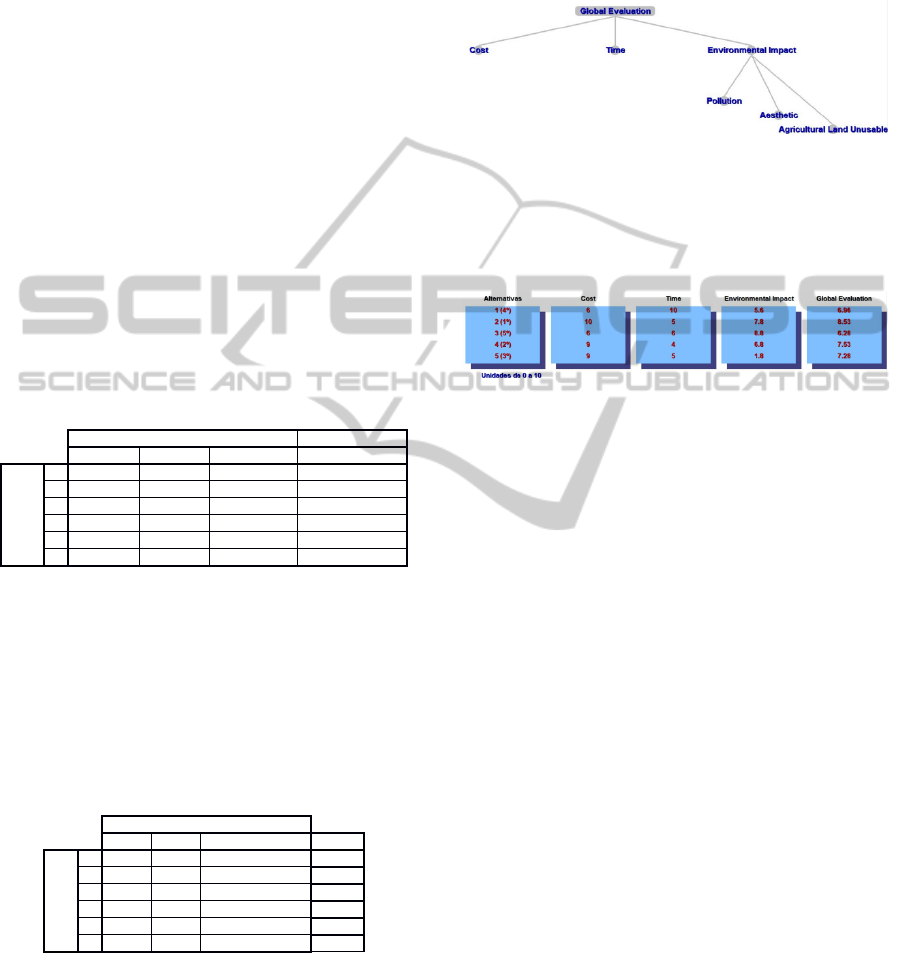
The criteria and sub criteria can be grouped as
illustrated in the figure below.
Figure 2: Representation of the criteria in tree, output
MacModel.
The table below shows the values entered in the
Software that proceeded immediately to the ordering
of the alternatives according to the weights above.
Figure 3: Output of MacModel already with the Global
Assessment for each alternative.
To define the lines of indifference we examine:
6
+10
+5.6
(
1−
−
)
=0.4
+4.4
+5.6
10
+5
+7.8
(
1−
−
)
=2.2
−2.8
+7.8
6
+6
+8.8
(
1−
−
)
=−2.8
−2.8
+8.8
⇔
−1.8
+7.2
=2.2
3.2
+7.2
=3.2
=15
⁄
The 1st equality refers to the tie between
locations 1 and 2.
The 2nd equality refers to the tie between
locations 1 and 3; finally the 3rd equality refers to
the tie between locations 2 and 3.
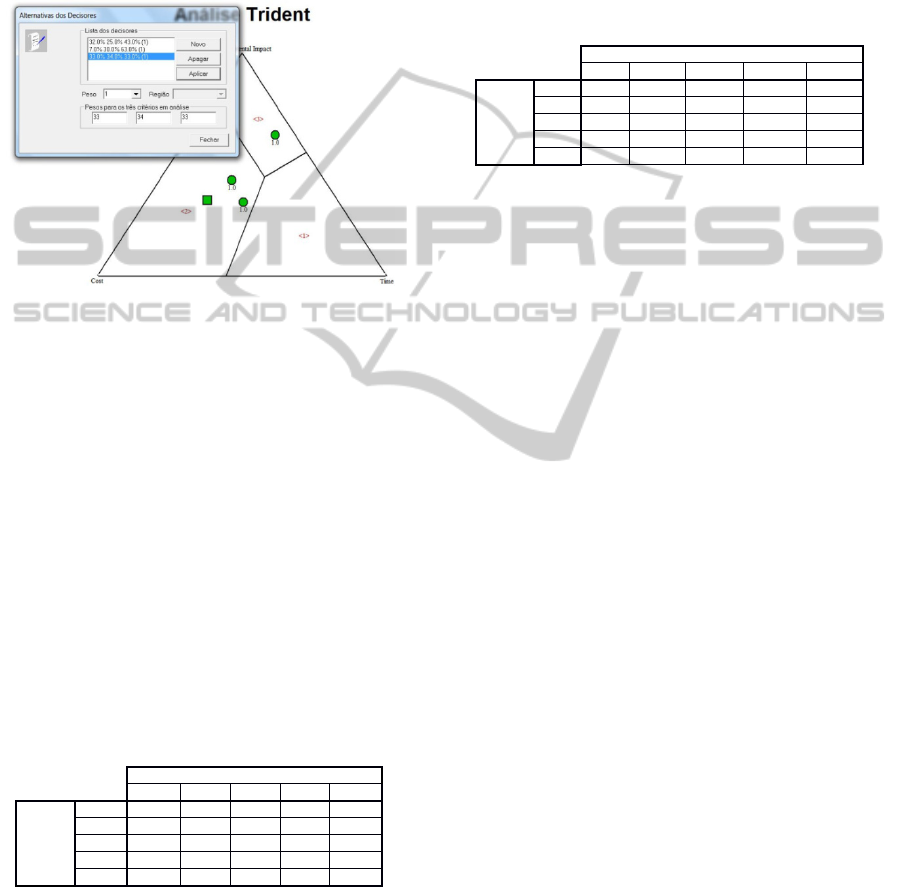
The sensitivity analysis of the weights can be
done using the Trident method (Valadares Tavares,
1984).
The decision should be made between the first
three locations. The location has a rating of 10 in a
time criterion while the second location has the
highest rating in the criteria cost. If greater weight is
given to the environmental impact criteria the
appropriate location is the 3.
Note that dominated alternatives, disappear in
the Trident analysis, since with any system of
weights they would never be in the first place.
Analyzing five alternatives (in which none is
dominated) analysis Trident shows five polygons.
INTRODUCTION TO MULTICRITERIA TECHNIQUES
493
At the other end if there is one that dominates all
others we will have a single region: the whole
triangle.
According to the weights assigned earlier 65%,
25% and 10% the decision is location 2.
One can also consider several decision makers and
get to the centroid of the most balanced solution as
illustrated in the following figure.
Figure 4: Output Analysis of MacModel with Trident,
when applied to multiple decision makers with different
weights assigned to the same criteria.
Continuing to analyze the same problem now we
apply the non-compensatory process Electre.
Electre is a non-compensatory method because it
is based on dichotomous comparisons, based on the
comparison between pairs of alternatives.
Infinitesimal changes of their values do not
change the final decision (provided they do not alter
the meaning of the order relation) as opposed to
compensatory model in which any change in
measurement changes the value.
1 - Matrix of agreement on what is considered
the same weights 65%, 25%, 10% and that means
how much better alternative is superior to the line of
the column.
Table 3: Matrix of Agreement.
Locations
1 2 3 4 5
Locations
1 0.25 0.9 0.25 0.35
2 0.75 0.65 1 1
3 0.75 0.35 0.35 0.35
4 0.75 0 0.65 0.75
5 0.65 0.25 0.65 0.9
The sum for each alternative in the matrix of
agreement is respectively 1.75, 3.4, 1.8, 2.15 and
2.45.
There is no doubt that the second alternative has
a higher value, such as in the compensatory model.
Alternative 5 has a high value because the
criterion with a big weight has a high value.
2 - Disagreement Matrix
It identifies all the alternatives now that the
Disagreement Matrix presents values greater than or
equal to 5. This is because we decided to veto all
alternatives that have a value greater than 5.
Note that a value of 5 in Matrix Disagreement is
equivalent to an increase of 5 on certain criteria.
Consequently we eliminate the alternatives 4 and 5.
Table 4: Matrix of Disagreement.
Locations
1 2 3 4 5
Locations
1 4 3.2 3 3
2 5 1 0 0
3 4 4 3 3
4 6 1 2 1
5 5 6 7 5
In all cases the matrix of disagreement has two
zeros at the same alternative so our present decision
is the best regardless of whether we want to apply a
method or the other (keeping the same weights).
REFERENCES
Coelho, José, 2001. MacModel multicriteria assessment,
in CESUR/IST, http://jcoelho.m6.net/ freeware/
MacModel2001.msi
Keeney, Ralph, 1988. Building Models of Values, European
Journal of Operational Research, 37:149-157.
Keeney, Ralph, 1992. Value Focus Thinking: A Path to
Creative Decision Making, Harvard University Press,
Cambridge, MA.
Roy, Bernard, 1968. Classement et choix en présence de
points de vue multiples (la méthode ELECTRE).
Revue d'Informatique et de Recherche Opérationelle
(RIRO), 8: 57–75.
Tavares, Valadares, 1984. The TRIDENT approach to
rank alternative tenders for large engineering projects,
Foundation of Control Engineering, 9(4):181-193.
Tavares, Valadares, Themido, I., Oliveira, R. and Correia,
F., 1996, Investigação Operacional, MacGraw-Hill.
ICORES 2012 - 1st International Conference on Operations Research and Enterprise Systems
494
