
HETEROGENEOUS ADABOOST WITH REAL-TIME
CONSTRAINTS
Application to the Detection of Pedestrians by Stereovision
Lo
¨
ıc Jourdheuil
1
, Nicolas Allezard
1
, Thierry Chateau
2
and Thierry Chesnais
1
1
CEA, LIST, Laboratoire Vision et Ing
´
enierie des Contenus, Gif-sur-Yvette, France
2
LASMEA, UMR UBP-CNRS 6602, 24 Avenue des Landais, Aubiere, France
Keywords:
Adaboost, Stereovision, Real Time.
Abstract:
This paper presents a learning based method for pedestrians detection, combining appearance and depth map
descriptors. Recent works have presented the added value of this combination. We propose two contributions:
1) a comparative study of various depth descriptors including a fast descriptor based on average depth in a
sub-window of the tested area and 2) an adaptation of the Adaboost algorithm in order to handle heteroge-
neous descriptors in terms of computational cost. Our goal is to build a detector balancing detection rate and
execution time. We show the relevance of the proposed algorithm on real video data.
1 INTRODUCTION
The pedestrian classification is one of the most re-
quested tools in the video surveillance field. Some
specific solutions exist in the context of video ac-
quired with stationary cameras. In this case, im-
age features from the spatial and temporal domains
are fused in order to jointly learn the correlation be-
tween appearance and foreground information based
on background subtraction (Yoa and Odobez, 2008).
Some other works (Dalal et al., 2006), (Wojek et al.,
2009) have used the fusion of the appearance and
movement in the image in order to improve results.
The method described in this article can not use
these combinations because its implementation field
is linked with the use of cameras embedded on mov-
ing vehicles. Issues linked with this class of appli-
cation are the reliability and the computing time of
the detector. During the last years, the community
has paid attention to depth map information coming
from sensors using stereovision (Walk et al., 2010),
(Enzweiler and Gavrila, 2011), (Ess et al., 2008),
in order to have an efficient classification. We will
present some of these descriptors and their perfor-
mances when they are used by an Adaboost learning
algorithm.
Works (Walk et al., 2010) combining both appear-
ance and disparity descriptors have been also pub-
lished recently. However, the fusion of several descr-
iptors often increases the processing time. In addi-
tion, this difference of computation time is never in-
cluded in the learning phase of the detector while the
objectives of the application are to achieve a real-time
solution. We propose a modification of Adaboost al-
gorithm by introducing a penalty linked with algorith-
mic complexity of each descriptor.
In a first part, we present different weak classi-
fiers based on depth information. Then we compare
them with the Histogram of Oriented Gradient (HOG)
method based on the image luminance. In a second
part, we will present an innovative learning method,
called Heterogeneous Adaboost (HAB), designed to
merge several detectors, by taking into account the
computing time of each algorithm.
2 DEPTH DESCRIPTORS
In this first section four descriptors of the depth map
are presented. The first three are based on local devia-
tions of depth. The last one is calculated on the depth
itself.
In the Figure 1, the left image shows a pedestrian
moving in an industrial environment. The pseudo im-
age on the right of the figure shows the representation
of the associated depth map.
The Figure 2 shows, in its upper part, a set of
depth maps for pedestrians (positive examples)and its
539
Jourdheuil L., Allezard N., Chateau T. and Chesnais T..
HETEROGENEOUS ADABOOST WITH REAL-TIME CONSTRAINTS - Application to the Detection of Pedestrians by Stereovision.
DOI: 10.5220/0003858305390546
In Proceedings of the International Conference on Computer Vision Theory and Applications (VISAPP-2012), pages 539-546
ISBN: 978-989-8565-03-7
Copyright
c
2012 SCITEPRESS (Science and Technology Publications, Lda.)
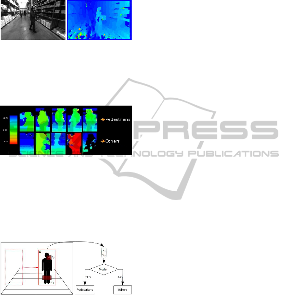
Figure 1: Example image (left) and the associated depth
map (right).
lower part examples of depth maps of the environment
(negative examples). The creation of this map is made
by a conventional method for dense depth map in real
time, not presented in this article.
Figure 2: Positive examples (upper) and negative examples
(lower) in the depth map.
A sliding window strategy (with a ratio of width
to height equals
1
2
) covering the ground level, is used
to scan the depth image ( Figure 3). For each window,
a feature vector composed a of set of local descriptors
from the depth map, is computed. Then vectors are
evaluated following a model created during off-line
learning stage.
Figure 3: Evaluation scheme of pedestrian classification.
2.1 Comparison of Descriptors
The use of depth map-based descriptors is recent. We
have adapted well-known efficient descriptors of ap-
pearance to be used on the depth map. We have also
created a specific descriptor of the depth map. We
present four depth map descriptors with HOG as a ref-
erence method on real images.
2.1.1 HOG-depth
This descriptor describes the depth map with as a His-
togram of Oriented Gradient (HOG) of depth. This
descriptor type is typically used to represent images
in appearance (Dalal and Triggs, 2005) generally. The
version used for the study, has been enriched with
the gradient magnitude, (Begard et al., 2008): a nor-
malized histogram of nine magnitudes of orientation
(from 0
◦
to 180
◦
) is built from the map of depth gra-
dient. Then this histogram is enriched with a tenth
value: the gradient magnitude.
2.1.2 Covariance Matrix (MatCov)
This descriptor, derived from the work of Tuzel (Tuzel
et al., 2008) offers a pedestrian coding from the co-
variance matrices of appearance and its spatial deriva-
tive, calculated on sub-windows of the scan. Our
proposition is the same as the previous one but using
information from the depth map with the data [x y d]
where x and y are the coordinates of pixel and d the
depth value of this pixel. Then the covariance matrix
is in a connected Riemannian manifold M
3×3
.
f
cov
: χ → M
3×3
(1)
Where M
3×3
is in R
3×3
. A function ψ : M
3×3
→ R
6
projects the manifold to the tangent space using the
formula:
ψ(X) = vec
µ
(log
µ
(X)) (2)
Where X and µ are two symmetric positive matrices.
With:
vec
µ
(X) = upper(µ
−
1
2
Xµ
−
1
2
) (3)
And :
log
µ
(X) = µ
1
2
log(µ
−
1
2
Xµ
−
1
2
)µ
1
2
(4)
µ is the point of the weighted average of the covari-
ance matrices, coming from the formula:
µ = arg min
Y ∈M
3×3
N
∑
i=1
d
2
(X
i
,Y ) (5)
So an essential metric for the comparison of the two
covariance matrices is defined.
2.1.3 Covariance, Depth Variance (CovVar)
The previous descriptor (MatCov) has the drawback
of being quite heavy in terms of computation time.
So one simplified version, consisting of the definition
of a distance which does not take any more account of
the properties of the Riemannian manifold, has been
used. In the covariance matrix 3 ∗ 3 created with the
data [x y d], the two first columns are constant. Thus,
the matrix is reduced to its last column and we get the
vector [cov(x, d) cov(y, d) var(d)]. So the norm L2
to define the distance between two descriptors can be
used by this reduction.
VISAPP 2012 - International Conference on Computer Vision Theory and Applications
540
2.1.4 Average
We propose a simple descriptor based on the average
of the differences between the test depth d and mea-
sured depth z in a sub-area of the window of analysis.
This descriptor called M
r
i
is associated with the re-
gion r
i
, and it is defined by the following equation:
M
r
i
=
1
n
∗
∑
d∈r
i
z − d if z defined
0 if z undefined
(6)
Where n is the number of defined depth points z. The
sizes and positions of regions r
i
are defined during the
learning phase.
This average depth-based descriptor may remem-
ber the descriptor DispStat (Walk et al., 2010) using a
fixed cutting up of the disparity map.
2.2 Performance Comparison
The performance comparison of the different descrip-
tors was done by using a learning machine type Adap-
tive Boosting algorithm (Freund and Schapire, 1999)
and a decision stump classifier type for HOG-depth,
CovVar, Average, and HOG on appearance. In the
case of a learning phase with MatCov, the weak clas-
sifier is a linear regression done on the components of
symmetric matrices.
2.2.1 Assessment Protocol
Learning has been done on a video shot inside a ware-
house where 10, 000 images of negative examples and
1, 500 images of positive examples have been ex-
tracted. Each tested area R is divided into 1, 482 rect-
angular regions r
i
.
In boosting methods, a new weak classifier is cho-
sen at each round of learning. Then the n chosen
weak classifiers are combined in a new strong classi-
fier. Each strong classifier is evaluated on 10, 000 im-
ages of negative examples and 1, 500 images of posi-
tive examples taken from a test video shot in a differ-
ent warehouse of this one the learning one. Following
tests done, the maximum of performance on the test
database can be achieved through a strong classifier,
created after the one which has reduced the learning
error to 0 in the learning phase. As about 100 rounds
of Adaboost are required by classifiers to reduce the
learning error to 0 on the learning database, we have
chosen to execute 300 rounds on the learning database
to maximize the probability of regulation of the max-
imum performance on the test database. The 300
Receiver Operating Characteristic (ROC) associated
with each classifier are compared and the best curve
is selected, according to the criterion:
Best = arg
300
max
t=1
Sur f ace(Curve
t
) (7)
Thus, each classifier type can be evaluated at its maxi-
mum performance regardless of the number of rounds
completed. A similar test of the HOG descriptor on
the appearance will be the reference curve.
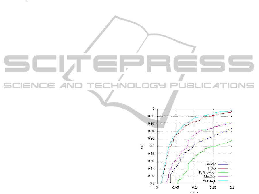
2.2.2 Results
The figure shows ROC curves obtained by using the
previous protocol. The curves have been compared at
a detection rate of 90% to the reference HOG curve
(red). HOG-Depth curve (green) has a false positive
rate of 15% or 11% above the baseline (4%). Strong
classifiers selected of curves HOG-Depth and HOG
have been learned with a respective number of rounds
of 270 and 290. The false positive rate of the curve
MatCov (purple) is 8% (120 rounds), the curve Cov-
Var (dark blue) is 10% (208 rounds), respectively 4%
and 6% higher than the reference. The percentage of
false positive of the Average curve (light blue) is close
to 4% (212 rounds) similar to the reference.
Figure 4: Comparison of detection performance of weak
classifiers on the depth map (HOG is the reference).
The results obtained using our Average classifier
created specifically to work on the depth map are as
good as the ones obtained using HOG appearance.
That confirms our initial hypothesis: the depth map
is sufficient to classify pedestrians. These encourag-
ing results, on the use of the depth map for the pedes-
trian classification, open a new way of merger with a
appearance descriptor.
HETEROGENEOUS ADABOOST WITH REAL-TIME CONSTRAINTS - Application to the Detection of Pedestrians by
Stereovision
541
3 HETEROGENEOUS
ADABOOST
The work (Walk et al., 2010) of Walker et al. has
shown that the fusion of descriptors of appearance,
motion and disparity improves significantly the clas-
sification results. However, this one generates an in-
crease in computing time which can be a limited fac-
tor not acceptable for real-time application.
In this second part, we propose to take account of
a constraint of algorithms cost, softened by α ∈ [0, 1],
in the Adaboost algorithm (Friedman et al., 1998)
(Heterogeneous Adaboost , HAB). It will be selec-
tion criteria of heterogeneous descriptors to create a
strong and fast classifier. Also, the depth descriptors
presented in the previous section, will be combined
with HOG appearance in a global learning phase.
Following the results of the previous study, the
method CovVar will be preferred to MatCov method
because the change of the method MatCov by CovVar
method damages a little bit results while reducing the
computation time.
3.1 Algorithm HAB
Let C be the set of weak learning algorithms to Ad-
aboost. We define an algorithm as a component de-
scriptors. We associate to each algorithm, its algorith-
mic cost λ
c
. The algorithmic cost can be estimated
from the complexity of the descriptor, or measured
statistically on a target machine.
One algorithmic cost softened normalized
˜
λ
c
, en-
abling management of the influence of algorithmic
cost in the calculation of the pseudo error penalized,
is calculated using the equation:
˜
λ
c
=
λ
α
c
∑
c=1,..,C
λ
α
c
(8)
where α ∈ [0; 1] is a softening coefficient choosen
empirically.
In the classical AdaBoost, the criterion to mini-
mize is calculated as follows:
ε
c
t
= E[e
−y
˜
h
c
t
] (9)
With
˜
h
c
t
: x → {−1;1} the response of the weak
classifier. We propose to penalize the criterion to min-
imize ε
c
t
by the algorithmic cost
˜
λ
c
in HAB. So the
new equation of the criterion to minimize (penalized)
becomes:
˜
ε
c
t
=
˜
λ
c
E[e
−y
˜
h
c
t
] (10)
When one component of a descriptor is chosen by
the algorithm, other ones related components of the
same descriptor are calculated simultaneously. There-
fore, the algorithmic cost λ
c
of all components of de-
scriptors already calculated change and should be up-
dated. So we introduced the algorithmic cost λ
0
of
classification without calculation.
For each component c already calculated, λ
c
is re-
placed by the algorithmic cost empty λ
0
. The new
normalized softened algorithmic cost
˜
λ
c
is recalcu-
lated.
Algorithm 1 on page 5 describes the different
stages of Heterogeneous Adaboost.
3.2 Algorithmic Cost
The evaluation of the complexity of the descriptor and
the statistical measure of processing time on a target
machine are among the possibilities to estimate the al-
gorithmic cost λ
c
of weak classifiers c ∈ C. We chose
to measure the average time (ns) of calculation re-
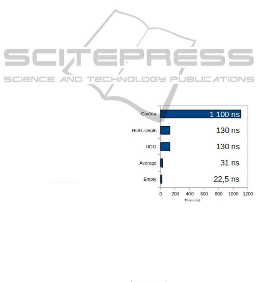
quired to calculate a weak classifier. The figure 5 rep-
resents the algorithmic cost
1
for each method CovVar,
HOG, HOG-depth and Average, and the algorithmic
cost (called empty) cited in the HAB algorithm, eval-
uated by a classifier that returns an empty vector.
Figure 5: Algorithmic cost λ
c
for each method Cov-
Var, HOG, HOG-depth and Average and empty cases in
nanoseconds (ns) per weak classifier.
The algorithmic cost varies from 1, 100ns for Cov-
Var to 31ns for the Average classifier which is close
to 22.5ns of the classifier empty. This classifier is
also four times faster than the reference HOG and its
derivative HOG-Depth (130ns).
We define the algorithmic cost Λ
t
of the strong
classifier output of the rounds t of HAB following
1
All tests were performed on a PC computer equipped
with a 2.8GHz processor.
VISAPP 2012 - International Conference on Computer Vision Theory and Applications
542

Algorithm 1: Heterogeneous Adaboost.
Require: N a set of labelled examples {(x
n
, y
n
)}
n=1,..,N
, D a probability distribution associated with N exam-
ples, C a set of learning algorithms with low computational cost associated {(WeakLearn
c
, λ
c
)}
c=1,..,C
, λ
0
algorithmic cost of empty, α ∈ [0;1] a coefficient of mitigations, T a number of iterations.
1: The weight vector w
1
i
= D(i) pour i = 1, .., N
2: A vector of normalized costs
˜
λ
c
=
λ
α
c
∑
c=1,..,C
λ
α
c
3: The initial error ε
0
= 0, 5
4: for t = 1 to T do
5:
w
t
=
w
t
∑
N
i=1
w
t
i
6: for c = 1 to C do
7: Call the weak classifier learner WeakLearn
c
with the distribution w
t
that returns a weak classifier
˜
h
c
t
=
1
2
P
w
t
(y=1|x)
P
w
t
(y=−1|x)
of algorithmic cost λ
c
.
8: Calculate the penalized criterion to minimize
˜
ε
c
t
=
˜
λ
c
E[e
−y
˜
h
c
t
]
9: end for
10: Select the weak classifier that minimizes the penalized criterion to minimize:
h
t
=
˜
h
ˆc
t
| ˆc = arg min
c=1,..,C
˜
ε
c
t
11: Update the weight vector
w
t+1
i
= w
t
i
e
−y
i
h
t
(x
i
)
12: Update of the new algorithmic cost λ
c
= λ
0
for all c calculated at the same time ˆc.
13: Normalization of the cost
˜
λ
c
=
λ
α
c
∑
c=1,..,C
λ
α
c
with α ∈ [0; 1]
14: end for
15: return the strong classifier:
H(x) = sign
"
T
∑
t=1
h
t
(x)
#
equation:
Λ
t
= Λ
t−1
+ λ
c
(11)
where λ
c
is the algorithmic cost of the weak classifier
selected round t.
3.3 Choice of the Softening Coefficient
α
The magnitude of the algorithmic cost
˜
λ
c
greatly in-
fluenced the choice of the weak classifier in the HAB
algorithm. To manage this influence, a softening coef-
ficient α is applied (equation 8). The latter is chosen
accordingly to the learning error and the computing
time Λ
t
.
In this section, we will present the influence
and the choice of a coefficient α for HAB with
HOG+Average descriptor.
3.3.1 Learning Error
The AdaBoost algorithm minimizes the learning error
for each of his rounds. The figure 6 shows the learning
error ε
t
based on the number of rounds t for classical
Adaboost (red) and the HAB algorithm (blue). As
we can see, the learning error of Adaboost is less the
HAB error.
In the figure 7, we represented the learning error
based on the algorithmic cost of strong classifiers Λ
t
(equation 11) to account for the algorithmic cost. In
this case, algorithm HAB (blue) reduces the learning
error faster than classical Adaboost (red) regardless of
the algorithmic cost (Time).
HETEROGENEOUS ADABOOST WITH REAL-TIME CONSTRAINTS - Application to the Detection of Pedestrians by
Stereovision
543
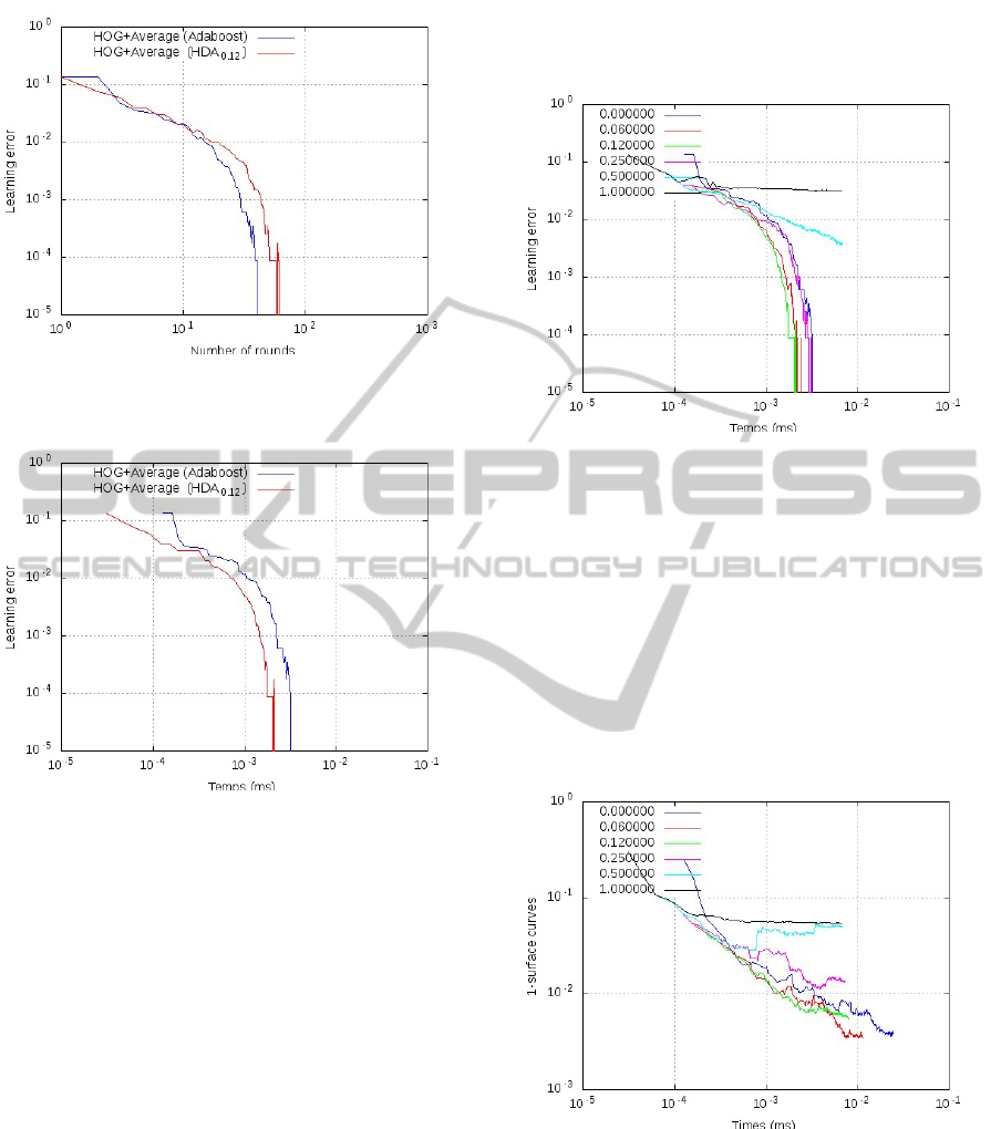
Figure 6: Learning error based on the number of rounds for
HOG+Average learning with classical Adaboost and HAB.
Figure 7: Learning error based on the number of comput-
ing time (ms) for learning HOG+Average with classical Ad-
aboost and HAB.
3.3.2 Determination of the Coefficient α
The experiments have showed that the algorithmic
cost influences strongly the selection of weak clas-
sifiers. We have looked for to manage its influence
by assigning a softening coefficient α (equation 8) to
it. The figure 8 shows the learning error based on the
algorithmic cost (time) for a representative sample of
possible values α ∈ {0; 0.06;0.12;0.25; 0.50; 1}. In
this figure, the curve α
1
(black) represents the learn-
ing error without softening coefficient. The percent-
age error of the learning curve has reached only 5%
error at the end of 300 rounds of learning. The curve
α
0
(dark blue) represents the evolution of the learning
error without algorithmic cost (softening maximum,
similar to a classical AdaBoost). The other curves
are related to values of the coefficient α ∈ [0; 1]. The
value of this coefficient has a very significant effect
on the performance of the algorithm. Curve α
0.12
(green) appears to be a good compromise between the
decrease of the learning error and computing time.
Figure 8: Learning error for HOG+Average
method based computation time (ms) for
α ∈ {0;0.06; 0.12; 0.25; 0.50; 1}.
To verify the effectiveness of the curve α
0.12
,
we used the data of the areas of ROC curves of
the protocol section 2.2.1 (page 3) that we posted
on a algorithmic cost Λ
t
. The figure 9 shows the
1-surface of the ROC curves as a function of time for
α ∈ {0; 0.06;0.12;0.25; 0.50; 1}.
It confirms the performance of the curve α
0.12
(green).
Figure 9: 1-surface curves ROC for HOG+Average
method based computation time (ms) for
α ∈ {0;0.06; 0.12; 0.25; 0.50; 1}.
3.4 Fixed Computation Time
This section presents the experiments conducted on
the test dataset, to compare method performance
with those of HAB on the three classical Adaboost
weak classifiers HOG+Average, HOG+CovVar et
VISAPP 2012 - International Conference on Computer Vision Theory and Applications
544
HOG+HOG-Depth. The protocol used is identical to
the one presented in section 2.2.1 (page 3). A maxi-
mum time limit lim for the time variable Λ
t
is defined
to reflect the real-time constraint.
Best = arg
300
max
t=1
Sur f ace(Curve
t
) if Λ
t
6 lim
0 if Λ
t
> lim
(12)
The time limit lim is set to 2.5µs and 1.25µs cor-
responding respectively to 10 and 20 frames per sec-
ond. This time limit has been estimated to account
for a number of 40, 000 tests sub-window to evalu-
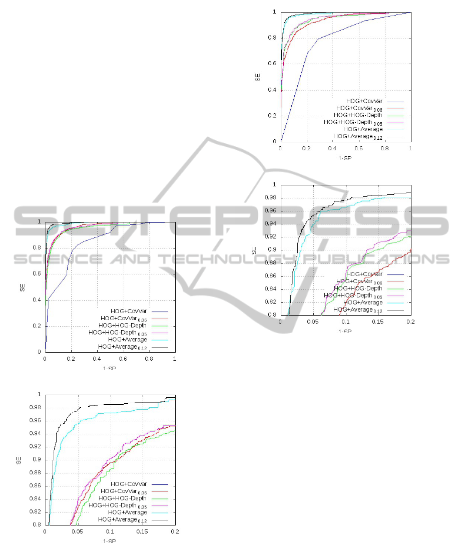
ate an image. Figure 10 (respectively 11) shows the
six ROC curves corresponding to lim = 2.5µs (respec-
tively lim = 1.25µs). Parts (a) represent the full curves
in the interval [0; 1] × [0;1], while parts (b) are zooms
in the interval [0; 0.2] × [0.8; 1].
(a) Interval [0;1] × [0; 1].
(b) Interval [0;0.2] × [0.8; 1].
Figure 10: ROC curves for comparison between a Ad-
aBoost and HAB for a computing time Λ
t
6 2.5µs.
In both figures, curves HOG+Average (light blue),
HOG+CovVar (dark blue) and HOG+HOG-Depth
(green) are learned with a classical Adaboost. The
(a) Interval [0;1] × [0; 1].
(b) Interval [0;0.2] × [0.8; 1].
Figure 11: ROC curves for comparison between a Ad-
aBoost and HAB for a computing time Λ
t
6 1.25µs.
others curves are learned with HAB and a coeffi-
cient α determined accordingly to the protocol pre-
sented above. The coefficient α is equal 0.12 for
HOG+Average (black), 0.06 for HOG+CovVar (red)
and 0.05 for HOG+HOG-Depth (purple). In both fig-
ures, the curves generated by HAB present a detec-
tion rate (SE) better than their counterparts produced
by classical Adaboost regardless of the false positive
rate (1-SP).
On the other hand, whatever the selected time, the
best strong classifier is given by HOG+Average learn-
ing (black).
The figure 4 (of page 3), showed that the CovVar
method is more efficient than HOG-Depth. However,
the CovVar algorithmic cost is ten times higher than
the HOG-Depth (figure 5). The figures 10 and 11
show that the merger by HAB leads to a combination
HOG+HOG-Depth that outperforms HOG+CovVar.
HETEROGENEOUS ADABOOST WITH REAL-TIME CONSTRAINTS - Application to the Detection of Pedestrians by
Stereovision
545

4 CONCLUSIONS AND
PROSPECTS
In this paper, in a first part, we have proposed and pre-
sented different descriptors of the depth map. Follow-
ing of the tests results the Average descriptor provides
performance equivalent to HOG descriptor which is
our reference.
In a second part, we have proposed a change of
the Adaboost algorithm taking account of the algo-
rithmic cost λ
c
for the selection of each weak classi-
fier. This new algorithm (HAB) has been evaluated on
the fusion of a appearance descriptor (HOG) with de-
scriptors of the depth map (CovVar, HOG-depth and
Average). The ROC curve which has a fixed process-
ing time, is superior to the conventional Adaboost ap-
proach. The output of HAB algorithm evaluates Al-
gorithms cost of strong classifier Λ
t
also.
The HAB algorithm could be adapted to the use
of a cascade (Viola and Jones, 2001) by setting a pro-
cessing time of each floor. In addition, the computa-
tional cost of each classifier can be redefined at each
stage in order to favour slow but efficient detectors at
the end of the cascade.
REFERENCES
Begard, J., Allezard, N., and Sayd, P. (2008). Real-time hu-
man detection in urban scenes: Local descriptors and
classifiers selection with adaboost-like algorithms. In
Computer Vision and Pattern Recognition Workshops,
2008. CVPRW ’08. IEEE Computer Society Confer-
ence on, pages 1–8.
Dalal, N. and Triggs, B. (2005). Histograms of oriented gra-
dients for human detection. In Computer Vision and
Pattern Recognition, 2005. CVPR 2005. IEEE Com-
puter Society Conference on, volume 1, pages 886–
893.
Dalal, N., Triggs, B., and Schmid, C. (2006). Human de-
tection using oriented histograms of flow and appear-
ance. In In European Conference on Computer Vision.
Springer.
Enzweiler, M. and Gavrila, D. (2011). A multilevel
mixture-of-experts framework for pedestrian classifi-
cation. Image Processing, 20(10):2967–2979.
Ess, A., Leibe, B., Schindler, K., , and van Gool, L. (2008).
A mobile vision system for robust multi-person track-
ing. In IEEE Conference on Computer Vision and Pat-
tern Recognition (CVPR’08). IEEE Press.
Freund, Y. and Schapire, R. E. (1999). A short introduction
to boosting. Journal of Japanese Society for Artificial
Intelligence, 14(5):771–780.
Friedman, J., Hastie, T., and Tibshirani, R. (1998). Addi-
tive logistic regression: a statistical view of boosting.
Statistics, Stanford University Technical Report.
Tuzel, O., Porikli, F., and Meer, P. (2008). Pedestrian
detection via classification on riemannian manifolds.
Transactions on Pattern Analysis and Machine Intel-
ligence, 30:1713–1727.
Viola, P. and Jones, M. (2001). Rapid object detection using
a boosted cascade of simple features. Computer Vision
and Pattern Recognition.
Walk, S., Schindler, K., and Schiele, B. (2010). Disparity
statistics for pedestrian detection: Combining appear-
ance, motion and stereo. ECCV, pages 182–195.
Wojek, C., Walk, S., and Schiele, B. (2009). Multi-cue on-
board pedestrian detection. In Computer Vision and
Pattern Recognition, 2009. CVPR 2009. IEEE Con-
ference on, pages 794–801.
Yoa, J. and Odobez, J. (2008). Fast human detection from
videos using covariance features. In 8th European
Conference on Computer Vision Visual Surveillance
workshop, Marseille.
VISAPP 2012 - International Conference on Computer Vision Theory and Applications
546
