
REAL-TIME POSE ESTIMATION USING TREE STRUCTURES
BUILT FROM SKELETONISED VOLUME SEQUENCES
Rune Havnung Bakken
1
and Adrian Hilton
2
1
Faculty of Informatics and e-Learning, Sør-Trøndelag University College, Trondheim, Norway
2
Centre for Vision, Speech and Signal Processing, University of Surrey, Guildford, U.K.
Keywords:
Human Motion, Pose Estimation, Real-time.
Abstract:
Pose estimation in the context of human motion analysis is the process of approximating the body configuration
in each frame of a motion sequence. We propose a novel pose estimation method based on constructing
tree structures from skeletonised visual hulls reconstructed from multi-view video. The pose is estimated
independently in each frame, so the method can recover from errors in previous frames, which overcomes the
problems of tracking. Publically available datasets were used to evaluate the method. On real data the method
performs at a framerate of 15–64 fps depending on the resolution of the volume. Using synthetic data the
positions of the extremities were determined with a mean error of 47–53 mm depending on the resolution.
1 INTRODUCTION
Capturing the motion of a person is a difficult task
with a number of useful applications. Motion capture
is used to identify people by their gait, for interact-
ing with computers using gestures, for improving the
performance of athletes, for diagnosis of orthopedic
patients, and for creating virtual characters with more
natural looking motions in movies and games. These
are but a few of the possible applications of human
motion capture.
In some of the application areas mentioned above
it is important that the data aquisition is unconstrained
by the markers or wearable sensors tradionally used
in commercial motion capture systems. Furthermore,
there is a need for low latency and real-time perfor-
mance in some applications, for instance in perceptive
user interfaces and gait recognition.
Computer vision based motion capture has been
a highly active field of research in the last couple
of decades, as surveys by for instance (Moeslund
et al., 2006) and (Poppe, 2007) show. A popular ap-
proach for multi-camera setups has been the shape-
from-silhouette method, which consists of doing 3D
reconstruction from silhouette images that results in
an over-estimate of the volume occupied by the sub-
ject called a visual hull.
Human motion is governed by an underlying artic-
ulated skeletal structure and (Moeslund et al., 2006)
define pose estimation as the process of finding an
approximate configuration of this structure in one or
more frames. In a tracking framework the temporal
relations between body parts during the motion se-
quence are ascertained. Many tracking based algo-
rithms suffer from increasing errors over time, and re-
covering from situations where the track is lost can be
problematic.
Goal. The overall goal of the research presented in
this paper is to develop a robust, real-time pose esti-
mation method.
Contribution. We present a pose estimation
method based on constructing a tree structure from
a skeletonised visual hull. The configuration of the
skeletal structure is independently estimated in each
frame, which overcomes limitations of tracking,
and facilitates automatic initialisation and recovery
from erroneous estimates. The method achieves
real-time performance on a variety of different
motion sequences.
This paper is organised as follows: in section 2
relevant work by other researchers is examined. The
proposed pose estimation method is detailed in sec-
tion 3. Results of experiments with the proposed
method are presented in section 4, and the strengths
and limitations of the approach are discussed in sec-
tion 5. Section 6 concludes the paper.
181
Havnung Bakken R. and Hilton A..
REAL-TIME POSE ESTIMATION USING TREE STRUCTURES BUILT FROM SKELETONISED VOLUME SEQUENCES.
DOI: 10.5220/0003858501810190
In Proceedings of the International Conference on Computer Vision Theory and Applications (VISAPP-2012), pages 181-190
ISBN: 978-989-8565-04-4
Copyright
c
2012 SCITEPRESS (Science and Technology Publications, Lda.)

2 RELATED WORK
The motion of the human body is governed by the
skeleton, a rigid, articulated structure. Recovering
this structure from image evidence is a common
approach in computer vision based motion capture.
Representing 3D objects by a skeletal approxima-
tion has many different applications. An overview of
the properties, applications and algorithms for finding
skeletal representations of 3D objects was given by
(Cornea et al., 2007). There are several ways to de-
fine the skeletal representation of an object. The well-
known medial axis transform (Blum, 1967) is used to
thin objects in 2D, but when generalised to 3D it re-
sults in a medial surface. The skeleton of an object is
defined as the locus of centre points of maximal in-
scribed balls. The medial axis and the skeleton are
closely related, but not exactly the same. The curve-
skeleton (Svensson et al., 2002) is an alternate repre-
sentation without a rigorous definition, but generally
it can be said to be a line-like 1D structure consisting
of curves that match the topology of the 3D object.
There exists a plethora of algorithms for finding
the curve-skeleton of an object, but (Cornea et al.,
2007) divides them into four broad categories: thin-
ning, geometrical, distance field, and potential field.
A thorough discussion of the strengths and weak-
nesses of each type of approach is beyond the scope
of this paper, but thinning offers a good compromise
between accuracy and computational cost. A subset
of the thinning category consists of fully parallel al-
gorithms. These procedures evaluate each voxel of
the 3D object independently, making them very well
suited for implementation on modern graphics hard-
ware.
Both (Brostow et al., 2004) and (Theobalt et al.,
2004) sought to find the skeletal articulation of arbi-
trary moving subjects. Both approaches enforce tem-
poral consistency for the entire structure during the
motion sequence. Neither focused on human pose es-
timation specifically, however, and no inferences were
made about which part of the extracted skeletons cor-
respond to limbs in a human skeletal structure.
A method for automatic initialisation based on
homeomorphic alignment of a data skeleton with a
weighted model tree was presented by (Raynal et al.,
2010). The alignment was done by minimising the
edit distance between the data and model trees. The
method was intended to be used as an initialisation
step for a pose estimation or tracking framework.
In the model-free motion capture method pro-
posed by (Chu et al., 2003) volume sequences are
transformed into a pose-invariant intrinsic space, re-
moving pose-dependent nonlinearities. Principal cu-
rves in the intrinsic space are then projected back
into Euclidean space to form a skeleton representation
of the subject. This approach requires three passes
through a pre-recorded volume sequence, hence it was
not suited for real-time applications.
Fitting a kinematic model to the skeletal data is
an approach taken by several researchers. The pose
estimation framework described by (Moschini and
Fusiello, 2009) used the hierarchical iterative closest
point algorithm to fit a stick figure model to a set of
data points on the skeleton curve. The method can
recover from errors in matching, but requires man-
ual initialisation. The approach presented by (Me-
nier et al., 2006) uses Delauney triangulation to ex-
tract a set of skeleton points from a closed surface vi-
sual hull representation. A generative skeletal model
is fitted to the data skeleton points using maximum
a posteriori estimation. The method is fairly robust,
even for sequences with fast motion. A tracking and
pose estimation framework where Laplacian Eigen-
maps were used to segment voxel data and extract a
skeletal structure consisting of spline curves was pre-
sented by (Sundaresan and Chellappa, 2008). Com-
mon for the three aforementioned approaches is that
they do not achieve real-time performance.
A comparison of real-time pose estimation meth-
ods was presented by (Michoud et al., 2007). Their
findings were that real-time initialisation was a fea-
ture lacking from other approaches. Michoud et al.’s
own approach has automatic initialisation and esti-
mates pose with a framerate of around 30 fps. It does,
however, rely on finding skin-coloured blobs in the vi-
sual hull to identify the face and hands, and this places
restrictions on the clothing of the subject and the start
pose, as well as requiring the camera system to be
colour calibrated.
The real-time tracking framework presented by
(Caillette et al., 2008) used variable length Markov
models. Basic motion patterns were extracted from
training sequences and used to train the classifier. The
method includes automatic initialisation and some de-
gree of recovery from errors, but as with all training
based approaches it is sensitive to over-fitting to the
training data, and recognition is limitied by the types
of motion that was used during the training phase.
3 APPROACH
In this section, we will detail the steps in the proposed
pose estimation method, starting with the input data,
and ending up with a set of labelled trees representing
the subject’s pose during the motion sequence.
VISAPP 2012 - International Conference on Computer Vision Theory and Applications
182

Table 1: Ratios of limb lengths in relation to the longest
path in the skeleton from one hand to one foot.
Bone Ratio Bone Ratio
Head 0.042 Upper spine 0.050
Upper neck 0.042 Lower spine 0.050
Lower neck 0.042 Hip 0.061
Shoulder 0.085 Thigh 0.172
Upper arm 0.124 Lower leg 0.184
Lower arm 0.121 Foot 0.050
Hand 0.029 Toe 0.025
Thorax 0.050
3.1 Anthropometric Measurements
In a fashion similar to (Chen and Chai, 2009) we build
a model of the human skeleton by parsing the data in
the CMU motion capture database (mocap.cs.cmu.
edu). The CMU database contains 2605 motion cap-
ture sequences of 144 subjects. For each sequence
the performer is described by an Acclaim skeleton file
that contains estimated bone lengths for 30 bones. We
parse all the skeleton files in the database and calcu-
late the mean bone lengths for a subset of the bones.
The stature was used as the reference length
when calculating anthromopometric ratios by (Mi-
choud et al., 2007), but as we wish to use these ra-
tios before the tree is labelled it is unknown which
parts of the tree constitute the stature. Hence, we need
an alternative reference length. We observe that the
longest path in the ideal tree structure in figure 1 is
from one hand to one foot (since the tree is symmetric
it does not matter which we choose). Consequently,
we use the longest path in the tree as the reference
length and it corresponds to the sum of the lengths of
the hand, lower and upper arm, thorax, lower and up-
per spine, hip, thigh, lower leg, foot, and toe. We cal-
culate the ratios for all limbs in relation to this longest
path. The limb length ratios are shown in table 1.
3.2 3D Reconstruction and
Skeletonisation
The first step in a shape-from-silhouette based ap-
proach is to separate foreground (subject) from back-
ground (everything else) in the image data. Both
the real and synthetic data used in this paper comes
with silhouette images already provided, so this step
is not included in the method, nor in the processing
times presented in section 4. There are, however, real-
time background subtraction algorithms available that
could be used. Any of the three methods examined by
(Fauske et al., 2009) achieve real-time performance
with reasonable segmentation results.
We assume that the camera system used is cali-
brated and synchronised. Experiments with multi-
camera systems by (Starck et al., 2009) demonstrated
that using eight or more cameras ensures good results
from the 3D reconstruction phase.
Once the silhouettes have been extracted the cali-
bration information from the cameras can be used to
perform a 3D reconstruction. The silhouette images
are cross sections of generalised cones with apexes in
the focal points of the cameras. The visual hull (Lau-
rentini, 1994) is created by intersecting the silhouette
cones. Visual hulls can be represented by surfaces
or volumes. We employ a simple algorithm that pro-
duces a volumetric visual hull. For all voxels in a
regular grid we project that voxel’s centre into each
image plane and check if the projected point is in-
side or outside the silhouette. Voxels that have pro-
jected points inside all the silhouettes are kept and the
rest are discarded. This procedure lacks the robust-
ness associated with more advanced techniques, but
its simplicity makes it attractive for implementation
on graphics hardware.
A parallel thinning technique (Bertrand and Cou-
prie, 2006) is used to skeletonise the visual hull. The
algorithm is implemented on graphics hardware to
achieve high throughput.
3.3 Pose Tree Construction
It is natural to represent the human body using a tree
structure. The head, torso and limbs form a tree-like
hierarchy. If the nodes in the tree are given positions
in Euclidean space the tree describes a unique pose.
3.3.1 Main Algorithm
An overview of the method can be seen in algo-
rithm 1. The first step is to create a tree structure
from the skeleleton voxels. A node is created for each
voxel, and neighbouring nodes are connected with
edges. Next, the extremities (hands, feet, and head)
are identified in the tree by first pruning away erro-
neous branches, and then examining branch lengths.
The third step consists of using the identified extrem-
ity nodes to segment the tree into body parts (arms,
legs, torso, and neck). Finally, a vector pointing for-
ward is estimated and used to label the hands and feet
as left or right. Further details about each step of the
method are given in the following sections.
3.3.2 Building the Tree
The skeleton voxel data is traversed in a breadth-first
manner to build the pose tree. We place the root of
the tree in the top-most voxel. The nodes are placed
REAL-TIME POSE ESTIMATION USING TREE STRUCTURES BUILT FROM SKELETONISED VOLUME
SEQUENCES
183

in a queue as they are created. When the first node in
the queue is removed the neighours of that node’s cor-
responding voxel is checked and new child nodes are
added to the tree if those neighbours have not been
visited before. This is repeated until the queue is
empty. At this point all voxels connected to the top-
most voxel will have been processed and given corre-
sponding nodes in the tree.
3.3.3 Finding Extremities
The next step is to identify the extremities among the
leaf nodes in the tree. The input skeleton voxels typ-
ically contain some noise which in turn leads to spu-
rious branches in the tree. Hence, we need to prune
the tree to reduce the number of leaf nodes. This is
done in two steps. First, a recursive procedure that
removes branches shorter than a threshold based on
the anthropometric ratios is employed. Calculating
the length of an arm with the anthropometric ratios
from section 3.1 and using that as the threshold has
been found to produce good results. Of the remain-
ing leaf nodes the feet should be at the end of the two
longest branches, and the hands should be at the end
of the next two. Hence, the list of leaf nodes is sorted
by branch length and all but the longest four are re-
moved. In order to keep all information in the origi-
nal tree intact the two pruning steps are performed on
a copy.
The procedure outlined above is robust as long as
Algorithm 1: Main pose estimation algorithm
1: Build the pose tree from skeleton voxels.
2: Find the extremities (feet, hands, head).
3: Segment the tree into body parts.
4: Find a vector pointing forward, and identify left
and right limbs.
Algorithm 2: A breadth-first pose tree construction algo-
rithm.
1: Create a node for the top-most voxel and add it to
the node queue.
2: while node queue is not empty do
3: N ← first node in queue.
4: V ← voxel corresponding to N.
5: for all neighbours of V do
6: if neighbour has not been visited then
7: Create a new child node of N and add it to
the queue.
8: Label neighbour as visited.
9: end if
10: end for
11: end while
the top-most voxel is at the location of the head. The
head branch is shorter than the length of an arm and
if one of the other limbs is higher than the head, the
head branch is likely to be removed during pruning.
We solve this problem by finding what we define as
the origin node.
Figure 1: An ideal pose tree. The black node is the origin
with degree four, the dark grey node is the root, the light
grey node is the internal node of degree three, and the white
nodes are leaf nodes. All other nodes are internal nodes of
degree two.
Let us consider an ideal pose tree. An ideal pose
tree consists of a root node, four leaf nodes, one inter-
nal node of degree three, one internal node of degree
four, and a number of internal nodes of degree two as
shown in figure 1. We define the origin node as the
node of degree four where the arms, torso, and neck
are joined.
All nodes in the pruned tree of degree higher than
two are candidates for the origin node. In order to
choose the best candidate we create copies of the
pruned tree and move the root to each of the candidate
locations. A rank is calculated for each of the candi-
date trees, and the root of the highest ranked tree is
chosen as the origin node.
The leaf nodes in the candidate tree are sorted by
distance to the root. The furthest two are used as feet,
the next two as hands, and the last as head. Ideal
lengths for the legs, arms, neck, and torso (I
l
,I
a
,I
n
,I
t
)
are estimated using the anthropometric ratios and the
longest path in the tree. We calculate the rank of a
candidate using the following formula:
r = r
l
1
·r
l
2
·r
a
1
·r
a
2
·r
n
·e
−
(deg(root)−4)
2
3
(1)
The last term is used to penalise candidate nodes
with degree 6= 4. The ranks for each limb is given by
the following formulae:
r
l
=
min(I
l
,d
r
)
max(I
l
,d
r
)
·
min(I
t
,d
r
−d
b
)
max(I
t
,d
r
−d
b
)
(2)
VISAPP 2012 - International Conference on Computer Vision Theory and Applications
184

Figure 2: Three candidates for the origin node of a tree
sorted by rank from left to right. Their ranks are 8.85 ×
10
−4
, 1.45 ×10
−4
, and 3.40 ×10
−5
, respectively.
r
a
=
min(I
a
,d
r
)
max(I
a
,d
r
)
·
1
1 + (d
r
−d
b
)
(3)
r
n
=
min(I
n
,d
r
)
max(I
n
,d
r
)
·
1
1 + (d
r
−d
b
)
(4)
where d
r
is the distance from the leaf node under con-
sideration to the root of the candidate tree, and d
b
is
the distance from the leaf node to the closest branch-
ing point. The second terms of equations 3 and 4 are
used to penalise candidates where one arm has been
shortened. An example of three candidate trees and
their ranks can be seen in figure 2.
The root of the pruned copy of the pose tree is
moved to the location of the highest ranked origin
candidate. If this is the first frame or no valid la-
belling is available from the previous frame, the leaf
nodes are sorted by the distance to the root. Finally,
the nodes in the original pose tree corresponding to
Algorithm 3: Finding extremities in the pose tree.
1: Create a copy of the tree.
2: Prune the copy by recursively removing branches
that are shorter than an arm.
3: Examine the remaining leaf nodes, and remove
all but the four belonging the longest branches
(feet and hands).
4: Create copies of the pruned tree with candidates
for the origin node position.
5: Rank the candidate trees and move the root of the
pruned copy to the location of the root of the can-
didate tree with the highest rank.
6: if no valid labelling from previous frame then
7: Sort leaf nodes by distance to root.
8: Label the furthest two as feet, the next two as
hands, and the final as head.
9: else
10: Label the leaf nodes by finding the nearest cor-
respondences from the previous frame.
11: end if
the remaining leaf nodes in the copy are labelled as
extremities. The two furthest from the root are la-
belled as feet, the next two as hands, and the last one
as the head.
If a valid labelling from the previous frame exists,
we use temporal correspondences to label the extrem-
ities instead. For each of the labelled extremities in
the previous frame, the Euclidean distance to each of
the remaining candidates in the current frame is calcu-
lated and the one with the shortest distance is chosen.
The chosen candidate is labelled correspondingly and
removed from the list of candidates.
If the head node is not the root of the tree, the root
is moved to that node. A lower limit on the origin
node rank is used to determine the validity of the la-
belling. This threshold is set empirically, and if none
of the candidate trees has a rank above the threshold
the labelling is not considered valid, and will not be
used for finding temporal correspondences in the next
frame.
3.3.4 Segmentation into Body Parts
Next, we segment the tree into body parts. The iden-
tified extremities are used as starting points for the
segmentation. Starting in the first hand node, the tree
is labelled as Arm1 upwards until the root is reached.
This is repeated for the other hand, and the tree is la-
belled as Arm2 upwards until the first node labelled
Arm1 is encountered. Labelling continues upwards,
and all nodes are labelled as Neck until the root is
reached. A similar approach is used for the lower
body. Starting in the first foot, the nodes are labelled
as Leg1 upwards in the tree until the label Neck is
reached. From the second foot, the nodes are labelled
as Leg2 upwards in the tree until the label Leg1 is en-
countered. Finally, continuing upwards, all nodes are
labelled as Torso until the label Neck is encountered.
If no nodes are labelled as Torso, the tree is marked as
invalid. This procedure is formalised in algorithm 4.
Algorithm 4: Tree segmentation (arms only; the legs, neck,
and torso are identified in a similar manner).
1: N ← the leaf node labelled Hand1.
2: while N is not the root do
3: Label N as Arm1.
4: N ← N’s parent.
5: end while
6: N ← the leaf node labelled Hand2.
7: while N is not labelled Arm1 do
8: Label N as Arm2.
9: N ← N’s parent.
10: end while
11: {Repeat for legs, neck and torso.}
REAL-TIME POSE ESTIMATION USING TREE STRUCTURES BUILT FROM SKELETONISED VOLUME
SEQUENCES
185

3.3.5 Identifying Left and Right
The final step of the proposed method is to find the
left and right sides of the body. We use the labelled
extremities as the starting point. Using the anthropo-
metric ratios from section 3.1 the algorithm creates
sets of nodes corresponding to the feet, lower legs,
thighs, and torso by traversing the tree upwards from
the labelled leaf nodes. Total least squares line fit-
ting is used to find vectors representing the node sets,
while making sure all vectors point upwards in the
tree.
Taking the cross products of the vectors, normal
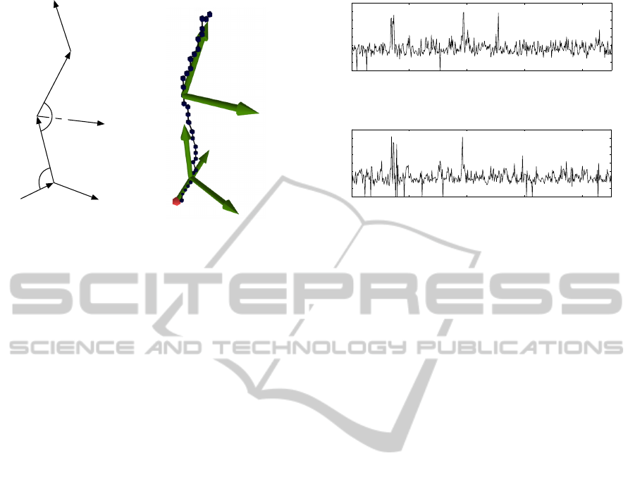
vectors for the ankle and joints are calculated. In fig-
ure 3(a) we observe that the angles α and β can never
exceed 180
◦
, so ordering the vectors in the cross-
product consistently ensures that the normals will be
oriented towards the left. For each leg the two joint
normals are combined to form a normal for the leg,
and a forward pointing vector for each leg is created
by taking the cross product of the normals and the
torso vector. The two forward vectors are combined
to form a single vector pointing forward in the torso’s
frame of reference. This procedure is formalised in
algorithm 5. Because of noise in the data it is possi-
ble that the foot can degenerate during the skeletoni-
sation and tree construction phases. In order to avoid
problems with the node sets used for the curve fitting,
a threshold is set on the difference in length between
the legs. If one leg is shorter by more than two times
the length of a foot, the foot vector and consequently
the ankle joint is disregarded in the calculation of the
normals.
To label the hands as left and right, total least
squares line fitting is used to find vectors representing
the shoulders, both pointing away from the torso. A
vector pointing left is calculated using the cross prod-
uct of the torso vector with the forward vector. The
angles between the shoulder vectors and the left vec-
tor is calculated, and the hand corresponding to the
smallest angle is labelled as left. If both shoulder vec-
tors are pointing in the same or opposite direction of
the left vector, the largest and smallest angle with the
forward vector, respectively, are used to label the left
hand. The procedure is repeated for the feet using
vectors representing the hips. The left-right labelling
is formalised in algorithm 6.
4 RESULTS
A number of experiments have been conducted using
the proposed method. Both real and synthetic data
were used, and reconstructions were done at resolu-
tions of 64 ×64×64 and 128 ×128×128 voxels. The
sizes of a voxel were 31.3 mm at 64 ×64 ×64, and
15.6 mm at 128 ×128 ×128. All experiments were
conducted on a computer with a 2.67 GHz Intel i7
Algorithm 5: Finding forward vector.
1: Using anthropometric ratios, create sets of nodes
corresponding to the foot, lower leg, thigh, and
torso.
2: Using orthogonal distance regression, fit lines to
the sets of nodes, and make sure the resulting vec-
tors ~v
f oot
,~v
lleg
,~v
thigh
,~v
torso
point upwards in the
tree.
3: if angle(~v
f oot
,~v
lleg
) > threshold then
4: Construct a normal for the ankle joint
~n
ankle
=~v
f oot
×~v
lleg
.
5: end if
6: if angle(~v
lleg
,~v
thigh
) > threshold then
7: Construct a normal for the knee joint
~n
knee
=~v
lleg
×−~v
thigh
.
8: end if
9: Combine the joint normals ~n
1
=
~n
ankle
+~n
knee
|~n
ankle
+~n
knee
|
.
10: Repeat step 3 to 9 for the other leg, to get a second
normal n
2
.
11: Construct two forward vectors using the normals
~
f
1
=~n
1
×~v
torso
.
12: Combine the two forward vectors
~
f =
~
f
1
+
~
f
2
|
~
f
1
+
~
f
2
|
.
Algorithm 6: Identifying left and right limbs.
1: For each arm, create a set of n nodes representing
the shoulder.
2: Construct a vector pointing left ~v
le f t
=~v
torso
×
~
f
3: Using orthogonal distance regression, fit lines to
the sets of nodes, and make sure the resulting vec-
tors ~v
1
and ~v
2
point away from the torso.
4: if ~v
le f t
·~v
1
> 0 and ~v
le f t
·~v
2
> 0 then
5: le f t = argmax(angle(
~
f ,~v
1
),angle(
~
f ,~v
2
))
6: right = argmin(angle(
~
f ,~v
1
),angle(
~
f ,~v
2
))
7: else if ~v
le f t
·~v
1
< 0 and ~v
le f t
·~v
2
< 0 then
8: le f t = argmin(angle(
~
f ,~v
1
),angle(
~
f ,~v
2
))
9: right = argmax(angle(
~
f ,~v
1
),angle(
~
f ,~v
2
))
10: else
11: le f t = argmin(angle(~v
le f t
,~v
1
),
angle(~v
le f t
,~v
2
))
12: right = argmax(angle(~v
le f t
,~v
1
),
angle(~v
le f t
,~v
2
))
13: end if
14: For each leg, create a set of n nodes representing
the hip, and repeat steps 3 to 12.
VISAPP 2012 - International Conference on Computer Vision Theory and Applications
186
↵
~v
foot
~v
foot
⇥~v
lleg
~v
lleg
~v
thigh
~v
lleg
⇥~v
thigh
~v
torso
(a) Joint angles and nor-
mals.
(b) Example using
real data.
Figure 3: Vectors used for left-right labelling.
processor, 12 GB RAM, and two graphics cards: one
Nvidia GeForce GTX 295 and one Nvidia GeForce
GTX 560 Ti. The GTX 295 was used for visual hull
construction and the GTX 560 for skeletonisation.
The accuracy of the method at different volume
resolutions was evaluated using synthetic data. An
avatar was animated using motion capture data from
the CMU dataset. Silhouette images of the sequence
were rendered with eight virtual cameras at a reso-
lution of 800 ×600, seven placed around the avatar
and one in the ceiling pointing down. The sequence
that was used was a whirling dance motion (subject
55, trial 1). The known joint locations from the mo-
tion capture data were used as a basis for compari-
son. The results of using the proposed pose estimation
method on the synthetic data can be seen in figure 4.
The mean positional error of the hands and feet for
the entire sequence was 46.8 mm (standard deviation
16.6 mm) and 53.2 mm (standard deviation 15.9 mm)
for 128 ×128 ×128 and 64 ×64 ×64 volume resolu-
tions, respectively. There is a noticeable increase in
accuracy with a higher resolution, but not by a huge
margin. An interesting observation is that the number
of frames where the method fails (curve reaches 0) in-
creases with higher resolution. The sequence consists
of 451 frames, and 97.6% and 95.8% are labelled cor-
rectly at 64×64×64 and 128×128×128 resolutions,
respectively.
The robustness and computational cost of the
method was evaluated using real data drawn from the
i3DPost dataset (Gkalelis et al., 2009). This is a pub-
lically available multi-view video dataset of a range
of different motions captured in a studio environment.
The volume resolution greatly influences the process-
ing time of the method. Three sequences of varying
complexity were tested at both 64×64×64 and 128×
100 200 300 400
Mean pos. error (mm)
Frame
0
120
80
40
160
(a) Volume resolution 64 ×64 ×64.
0
120
80
40
160
100 200 300 400
Frame
Mean pos. error (mm)
(b) Volume resolution 128 ×128 ×128.
Figure 4: Comparison of mean errors of estimated posi-
tions of the hands and feet for a synthetic dance sequence.
Frames where the algorithm has failed gracefully have been
omitted.
128 ×128 resolutions, and the results can be seen in
table 2. The method achieves near real-time perfor-
mance of ∼ 15 fps at the highest resolution, but by
halving the dimensions of the volume the framerate is
almost tripled. A framerate of ∼64 fps should be suf-
ficient for most real-time applications. In both cases
the tree construction is highly efficient, < 1.5 ms for
64 ×64 ×64 and < 4 ms for 128 ×128 ×128. At
the higher resolution the skeletonisation is the main
computational bottleneck. The reason for the small
difference in processing time for the visual hull con-
struction is that the images from the i3DPost dataset
have a resolution of 1920×1080 and copying the data
between main memory and the GPU is the bottleneck.
Figure 5 shows four frames from the three sequences
at both resolutions.
Sequences with challenging motions were used to
test the robustness. Poses where the subject’s limbs
are close to the body typically result in a visual hull
that is a poorer approximation of the actual volume.
A sequence where the subject is crouching during the
motion illustrates this. As can be seen in figure 6 the
method fails gracefully when the subject is crouching,
but recovers once the limbs are spread out once more.
A pirouette is a challenging motion, because of the
rapid movement of the extremities. Figure 7 shows
that the temporal correspondence labelling can fail in
such cases, but the identification of the left and right
limbs is still robust.
For the real data, the walk (57 frames) and
walk-spin (46 frames) sequences are labelled 100%
correctly. Only 42.6% of the run-crouch-jump (108
frames) sequence is labelled correctly, but the subject
is crouching during half the sequence. The sequences
REAL-TIME POSE ESTIMATION USING TREE STRUCTURES BUILT FROM SKELETONISED VOLUME
SEQUENCES
187
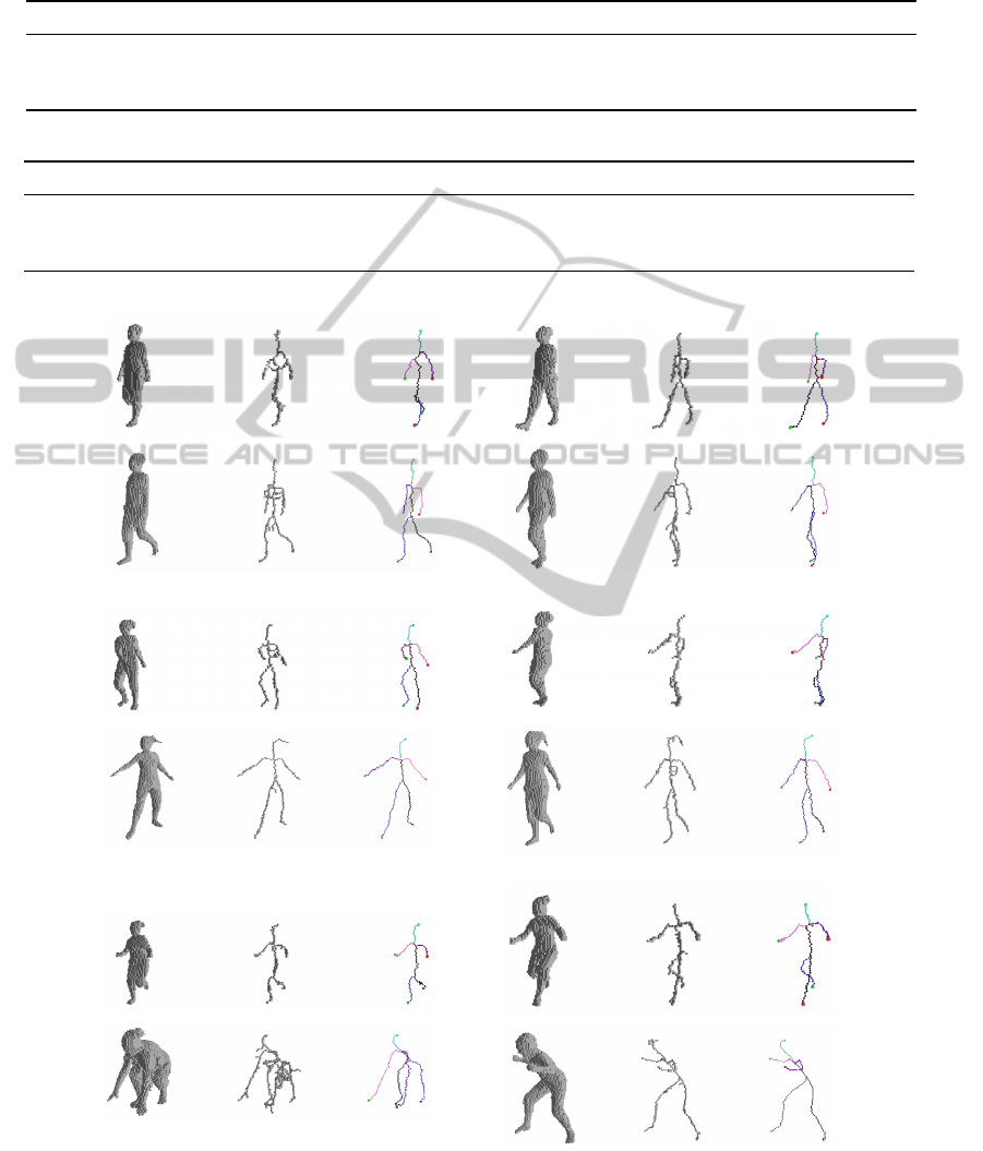
Table 2: Comparison of mean processing times for three sequences from the i3DPost dataset, using different resolutions. All
times are in milliseconds, with standard deviations in parentheses.
(a) Volume resolution 64 ×64 ×64.
Visual hull Skeletonisation Build tree Sum Framerate
Walk, sequence 013 9.61 (0.26) 4.37 (0.28) 1.44 (0.25) 15.41 (0.47) 64.88
Walk-spin, sequence 015 9.63 (0.26) 4.42 (0.32) 1.41 (0.30) 15.46 (0.54) 64.67
Run-crouch-jump, sequence 017 9.69 (0.26) 4.82 (0.59) 1.07 (0.27) 15.58 (0.61) 64.18
(b) Volume resolution 128 ×128 ×128.
Visual hull Skeletonisation Build tree Sum Framerate
Walk, sequence 013 12.25 (0.34) 49.37 (2.63) 3.09 (0.33) 64.71 (2.61) 15.45
Walk-spin, sequence 015 12.28 (0.30) 52.06 (4.14) 3.13 (0.46) 67.46 (4.03) 14.82
Run-crouch-jump, sequence 017 11.94 (0.16) 51.43 (3.73) 3.51 (0.58) 66.88 (3.89) 14.95
(a) Walk, sequence 013.
(b) Walk-spin, sequence 015.
(c) Run-crouch-jump, sequence 017.
Figure 5: Four frames from each of three sequences, showing the visual hulls, skeletons and pose trees. The top rows have a
volume resolution of 64 ×64 ×64, and 128 ×128 ×128 in the bottom rows.
VISAPP 2012 - International Conference on Computer Vision Theory and Applications
188
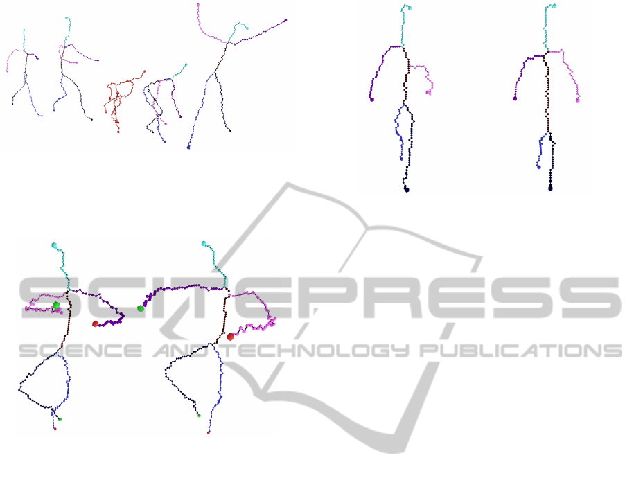
Figure 6: Five frames from the run-crouch-jump sequence
(017 from the i3DPost dataset) illustrating the problems that
occur when the subject is crouching and no reliable skeleton
can be extracted, but also that the algorithm recovers when
the arms and legs become distinguishable again.
Figure 7: Two consecutive frames of a ballet sequence (023
of the i3DPost dataset) where the correspondence labelling
has failed and the arm colours have switched sides. The
left-right labelling, however, is still correct as illustrated by
the red and green extremities.
were truncated to keep the subject completely inside
the viewing volume. The ballet sequence consists
of 150 frames and 87.3% of them were labelled cor-
rectly.
5 DISCUSSION AND FUTURE
WORK
In the previous section we demonstrated the proposed
method on several sequences where it robustly recov-
ers a segmented skeletal structure. There are, how-
ever, some limitations to using a skeletonisation based
approach, and we will discuss them here, and how
these issues can be resolved in the future.
Cases can be found that are likely to be problem-
atic for a skeletonisation based method. The extracted
skeleton is unreliable in frames where the limbs are
not clearly separated from the rest of the body. How-
ever, it is possible to detect these cases and give
an indication that the pose estimate for that partic-
Figure 8: Two frames of a walk sequence (013 from the
i3DPost dataset) demonstrating the possible displacement
of the shoulders and the pelvis. The proposed method com-
pensates for this, and the limbs are still labeled correctly.
ular frame is not trustworthy. A significant advan-
tage of the proposed approach is that the skeleton in
each frame can be labelled independently of previ-
ous frames. As was demonstrated in section 4 this
allows the approach to recover from errors in previ-
ous frames where the skeletal reconstruction may be
degenerate.
In figure 8 we see a common problem with us-
ing the curve-skeleton. In frames where the arms are
close to the torso or the legs are too close to each
other, the shoulders and pelvis tend to be displaced
downwards. This is not a major issue for the proposed
algorithm, but it is important to keep in mind if more
joint locations should be extracted in the future.
The lower limit on the rank of candidate trees we
use to determine a labelling’s validity is heuristic, and
a better alternative should be found. Though the em-
pirically set threshold works for the sequences we
have tested with, there are no guarantees that it will
do so for other data.
Currently, only the locations of the hands, feet,
and the head are estimated. We intend to extend the
method with estimates for the positions of internal
joints as well. Creating a kinematic model using the
limb length ratios in section 3.1 and fitting that to the
skeleton data is an approach that will be examined fur-
ther.
In order to better compare the proposed approach
to other methods that attempt to solve the pose esti-
mation problem, the method should be tested on more
publically available datasets, for instance HumanEVA
or INRIA IXMAS.
REAL-TIME POSE ESTIMATION USING TREE STRUCTURES BUILT FROM SKELETONISED VOLUME
SEQUENCES
189

6 CONCLUDING REMARKS
We have presented a novel pose estimation method
based on constructing tree structures from skele-
tonised sequences of visual hulls. The trees are
pruned, segmented into body parts, and the extrem-
ities are identified. This is intended to be a real-
time approach for pose estimation, the results for
the pose tree computation back this up and demon-
strate good labellings across multiple sequences with
complex motion. The approach can recover from er-
rors or degeneracies in the initial volume/skeletal re-
construction which overcomes inherent limitatons of
many tracking approaches which cannot re-initialise.
Ground-truth evaluation on synthetic data indicates
correct extremity labelling in ∼ 95% of frames with
rms errors < 5 cm.
ACKNOWLEDGEMENTS
The authors wish to thank Lars M. Eliassen for help-
ing with the implementation of the skeletonisation
algorithm, and Odd Erik Gundersen for his helpful
comments during the writing of the paper. Some of
the data used in this project was obtained from mo-
cap.cs.cmu.edu. The CMU database was created with
funding from NSF EIA-0196217.
REFERENCES
Bertrand, G. and Couprie, M. (2006). A New 3D Parallel
Thinning Scheme Based on Critical Kernels. Discrete
Geometry for Computer Imagery (LNCS), 4245:580–
591.
Blum, H. (1967). A transformation for extracting new de-
scriptors of shape. Models for the perception of speech
and visual form, 19(5):362–380.
Brostow, G. J., Essa, I., Steedly, D., and Kwatra, V. (2004).
Novel skeletal representation for articulated creatures.
Computer Vision - ECCV (LNCS), 3023:66–78.
Caillette, F., Galata, A., and Howard, T. (2008). Real-time
3-D human body tracking using learnt models of be-
haviour. Computer Vision and Image Understanding,
109(2):112–125.
Chen, Y.-l. and Chai, J. (2009). 3D Reconstruction
of Human Motion and Skeleton from Uncalibrated
Monocular Video. Computer Vision - ACCV (LNCS),
5994:71–82.
Chu, C.-W., Jenkins, O. C., and Mataric, M. J. (2003).
Markerless Kinematic Model and Motion Capture
from Volume Sequences. In Proceedings of the IEEE
Conference on Computer Vision and Pattern Recogni-
tion, pages 475–482.
Cornea, N. D., Silver, D., and Min, P. (2007). Curve-
Skeleton Properties, Applications, and Algorithms.
IEEE Transactions on Visualization and Computer
Graphics, 13(3):530–548.
Fauske, E., Eliassen, L. M., and Bakken, R. H. (2009).
A Comparison of Learning Based Background Sub-
traction Techniques Implemented in CUDA. In Pro-
ceedings of the First Norwegian Artificial Intelligence
Symposium, pages 181–192.
Gkalelis, N., Kim, H., Hilton, A., Nikolaidis, N., and Pitas,
I. (2009). The i3DPost multi-view and 3D human ac-
tion/interaction database. In Proceedings of the Con-
ference for Visual Media Production, pages 159–168.
Laurentini, A. (1994). The Visual Hull Concept for
Silhouette-Based Image Understanding. IEEE Trans-
actions on Pattern Analysis and Machine Intelligence,
16(2):150–162.
Menier, C., Boyer, E., and Raffin, B. (2006). 3D Skeleton-
Based Body Pose Recovery. In Proceedings of the
Third International Symposium on 3D Data Process-
ing, Visualization, and Transmission, pages 389–396.
Michoud, B., Guillou, E., and Bouakaz, S. (2007). Real-
time and markerless 3D human motion capture us-
ing multiple views. Human Motion - Understanding,
Modeling, Capture and Animation (LNCS), 4814:88–
103.
Moeslund, T. B., Hilton, A., and Krüger, V. (2006). A sur-
vey of advances in vision-based human motion cap-
ture and analysis. Computer Vision and Image Under-
standing, 104:90–126.
Moschini, D. and Fusiello, A. (2009). Tracking Human
Motion with Multiple Cameras Using an Articulated
Model. Computer Vision/Computer Graphics Collab-
oration Techniques (LNCS), 5496:1–12.
Poppe, R. (2007). Vision-based human motion analysis: An
overview. Computer Vision and Image Understand-
ing, 108(1-2):4–18.
Raynal, B., Couprie, M., and Nozick, V. (2010). Generic
Initialization for Motion Capture from 3D Shape. Im-
age Analysis and Recognition (LNCS), 6111:306–315.
Starck, J., Maki, A., Nobuhara, S., Hilton, A., and Mat-
suyama, T. (2009). The Multiple-Camera 3-D Pro-
duction Studio. IEEE Transactions on Circuits and
Systems for Video Technology, 19(6):856–869.
Sundaresan, A. and Chellappa, R. (2008). Model-driven
segmentation of articulating humans in Laplacian
Eigenspace. IEEE Transactions on Pattern Analysis
and Machine Intelligence, 30(10):1771–1785.
Svensson, S., Nyström, I., and Sanniti di Baja, G. (2002).
Curve skeletonization of surface-like objects in 3D
images guided by voxel classification. Pattern Recog-
nition Letters, 23:1419–1426.
Theobalt, C., de Aguiar, E., Magnor, M. A., Theisel, H., and
Seidel, H.-P. (2004). Marker-free kinematic skeleton
estimation from sequences of volume data. Proceed-
ings of the ACM symposium on Virtual reality software
and technology - VRST ’04, D:57.
VISAPP 2012 - International Conference on Computer Vision Theory and Applications
190
