
ALGORITHM TO MAINTAIN LINEAR ELEMENT IN 3D LEVEL
SET TOPOLOGY OPTIMIZATION
Christopher J. Brampton, Alicia H. Kim and James L. Cunningham
Department of Mechanical Engineering, University of Bath, Bath, U.K.
Keywords: Level set method, 3D topology optimization, Voxel mesh.
Abstract: In level set topology optimization the boundary of the structure is defined by level set function values stored
at the nodes of a regular gird of simple bilinear elements. By changing the level set function values
according to optimization sensitivities the boundary of the structure is moved to create an optimal structure.
However it is possible for the boundary to cut an element more than once; violating the linear element
assumptions resulting in insufficient nodal information for the optimization sensitivity calculations. To
resolve this the local boundary of the structure is moved so that each element is only cut once. In 2D where
a square element mesh is used an element cut twice times is altered by moving one of the boundaries within
the element to intercept the node closest to it removing the extra cut from the element. In 3D where a voxel
mesh is used the process of moving the boundary within an element is more complicated due to the greater
number of boundary cuts possible and the effect that it can have on neighbouring elements. An algorithm is
developed which allows the boundary within a 3D element to be moved with these considerations taken into
account.
1 INTRODUCTION
Topology optimization is considered to have enabled
a step-change in structural design as it is the most
generalized form of structural optimization
producing a solution least dependent on the initial
design. It usually starts with a continuum of the
available design space and finds the optimal
topology as well as shape and size of the structural
members within it. One parameterization that is
receiving much interest in recent years is the level
set method due to its flexibility and stability in
handling topological changes (Allaire et al., 2004).
Topology optimization is an iterative process
where a finite element analysis is applied to carry
out the sensitivity analysis. The local sensitivities
are then used to update the level set function values,
thus modifying the structural boundaries to create an
improved structural geometry. To avoid the need for
a new finite element mesh every iteration the
geometry is usually projected onto a regular mesh of
elements (Allaire et al., 2004). Since the finite
element analysis is the computational bottleneck of
optimisation simple 1
st
order bilinear elements (4
node rectangular elements in 2D and 8 node brick
elements in 3D) are most commonly used in
topology optimisation (Dunning and Kim, 2011).
For convenience finite element nodes are used to
define the level set function. As the geometric
boundary defined by the level set function does not
always conform to the regular element edges, there
is a group of boundary elements which are cut by the
boundary. A variety of methods have been used to
estimate the material properties of these elements,
from simple element volume ratio based calculations
(Allaire et al., 2004) (Jang and Kim, 2005) (Wang et
al., 2007) to local remeshing approaches (Wang and
Wang, 2006).
A popular approach is to compute local
sensitivities per element for the level set function
update (Allaire et al., 2004) (Jang and Kim, 2005).
This means the elemental properties are
homogenised and the nodal properties are
approximately computed by interpolating the
elemental properties, instead of using the more
accurate nodal values from finite element analysis.
Nodal sensitivities can be used directly to update the
level set function (Dunning and Kim, 2011).
However this means an element can be cut by two
boundaries. In these cases, there are insufficient
nodes for the subsequent finite element analysis to
describe the linear displacement field of the element,
341
J. Brampton C., H. Kim A. and L. Cunningham J..
ALGORITHM TO MAINTAIN LINEAR ELEMENT IN 3D LEVEL SET TOPOLOGY OPTIMIZATION.
DOI: 10.5220/0003860003410350
In Proceedings of the 1st International Conference on Pattern Recognition Applications and Methods (SADM-2012), pages 341-350
ISBN: 978-989-8425-98-0
Copyright
c
2012 SCITEPRESS (Science and Technology Publications, Lda.)

thus sensitivities cannot be computed for the next
iteration.
Several methods have been devised to resolve
the problem of elements containing multiple
boundaries. The simplest is to declare cut elements
to be entirely outside the structure (Challis, 2010),
however this is a significant simplification and
increases the mesh density required for accurate
optimization. Researchers have employed the
extended finite element method (X-FEM). This has
been developed primarily for describing fractures
and multi-scale analysis where the elemental
stiffness matrix is “enriched” to describe the local
material distribution. However, higher order
elements must be used at the geometric boundary to
accomplish this (Belytschko et al., 2003) (Wei et al.,
2010). The local mesh refinement method splits each
cut element into multiple elements which are fitted
to the geometric boundary (Wang and Wang, 2006).
However both these methods require an increase of
the degrees of freedom with considerable additional
computation. This increases the computational cost
of the finite element analysis which is already a
processing bottle neck.
This paper proposes an alternative method to
resolve the problem of elements containing multiple
cuts without increasing the degrees of freedom in the
finite element model. The proposed approach is to
alter the local boundary geometry so that no
elements contain multiple boundaries allowing first
order bilinear elements to be used on the geometric
boundary. This allows the use of accurate nodal
properties to compute the sensitivities and avoids the
unnecessary additional computational complexity.
The numerical results show that the boundary “fix”
proposed in this paper is sufficiently minimal and
the algorithm consistently finds the optimum
solutions.
2 BOUNDARY MODIFICATION
IN 2D
2.1 Problem Statement
The level set topology optimization procedure
moves the structural boundary by cutting through
elements. As a result it is possible for multiple
boundaries to simultaneous cut through an element.
When 1
st
order elements are used, there is
insufficient nodal information for sensitivity
computation in elements containing multiple
boundary cuts and thus, they are considered
“illegal”. In order to proceed with the topology
optimization procedure any illegal elements must be
avoided.
In 2D this occurs when an element is cut twice,
usually due to a narrow strut or a small hole in the
structure. An example of a legal and illegal element
can be seen in Figures 1 and 2, respectively.
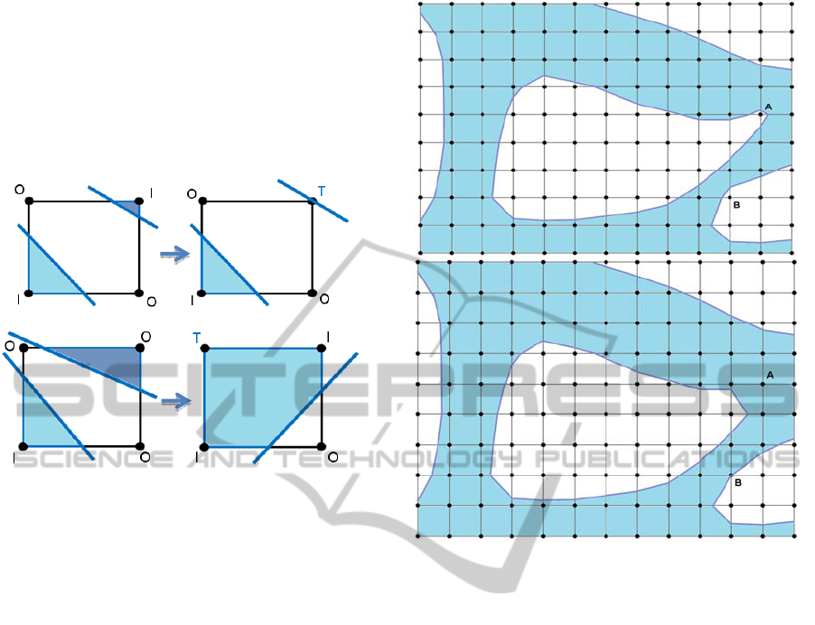
Figure 1: Legal 2D Element. The structure is indicated by
the shaded region.
Figure 2: Illegal 2D Element.
2.2 Treatment for Illegal Elements
A simple and computationally efficient method is to
move the boundary such that all elements contain a
maximum of one cut. To identify the illegal
elements we examine the status of the element
nodes.
The implicit level set function representation
usually has two node statuses, a node is inside the
structure (an I-node) if the level set function is
positive and is outside the structure (an O-node) if
the level set function is negative. An element is cut
by the boundary if it is made of both I-nodes and O-
nodes. Similarly an edge of the element is cut if it
has an I-node on one end and an O-node on the
other. In 2D an element is considered illegal if an
element contains two I-nodes and O-nodes in
opposite corners as seen in Figure 2. In this case the
element contains more than two cut edges, this
identifies an illegal element in 2D.
We introduce a new node status, a touching node
(a T-node) that is considered to be exactly on the
boundary of the structure. A T-node can be either
inside or outside depending on the status of the
nodes it shares an edge with. If a T-node shares an
ICPRAM 2012 - International Conference on Pattern Recognition Applications and Methods
342
edge with an I-node the edge is inside the structure,
if it shares an edge with an O-node the edge is
outside the structure. Hence, a T-node is inside the
structure if both edges it is connected to are inside
and outside if both edges it is joined to are outside.
If one edge is outside the structure and the other
inside the structure the boundary intercepts the T-
node.
Figure 3: Examples of boundary updates to avoid illegal
elements using T-nodes. The illegal elements on the left
and modified legal elements on the right.
By changing an I-node or O-node in an illegal
element to a T-node the boundary immediately
adjacent to the T-node is moved as shown in Figure
3. This moves the boundary outside the element so
that it no longer cuts the neighbouring edges and
only one boundary remains, making the element
legal. To minimize the modification, the node that is
the shortest distance away from the boundary, as
defined by its level set function value, is selected to
be changed to a T-node.
This boundary modification algorithm is applied
every iteration after an optimization step and Figure
4 shows an example of the effect it can have on the
topological solution. In order to minimize the effects
of this algorithm on the overall optimization
procedure, it is assumed that the mesh density is of a
reasonable density.
3 BOUNDARY MODIFICATION
IN 3D
The additional dimension in 3D level set topology
optimization significantly increases the complexity
of the necessary algorithm both to identify and
eliminate the illegal elements. To achieve robust
treatment of illegal 3D elements a more advanced
Figure 4: An example of how treating an illegal element
affects the global structure. Nodes A and B are changed to
T-nodes. The mesh density should be high enough for
these features to be considered to be minimal.
correction method is formulated as discussed in the
following.
3.1 Identification of Illegal 3D
Elements
A 3D element is considered illegal if a boundary of
the structure cuts the element in a manner that
cannot be represented by a single linear cut. Again
this occurs when the boundary of the structure cuts
an element more than once. Figure 5 shows
examples of legally cut 3D elements and Figure 6
features examples of illegal elements showing that in
3D between two and four separate cuts by the
boundary are possible. This complicates the
detection of illegal elements as there is not a clear
relationship between the number of cut edges and
the illegal elements. While the maximum number of
cut edges in a legal element is 6 (Figure 5), the same
number of cuts can produce an illegal element
(Figure 6). Introducing T-nodes does not lead to a
well-defined relationship between the number of cut
edges and illegal elements, as shown in Figure 7.
ALGORITHM TO MAINTAIN LINEAR ELEMENT IN 3D LEVEL SET TOPOLOGY OPTIMIZATION
343
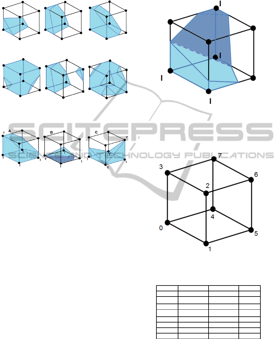
Figure 5: Examples of legally cut 3D elements.
Figure 6: Example of illegal 3D elements that have been
cut more than once. It is possible for an element to be cut
four times.
Figure 7: Example of 3D elements containing T-nodes.
Element A is legal. Elements B and C illegal are as the T-
nodes are intercepted by the boundary within the element
in a manner that cuts the volume of material in two.
Another approach that could be used to identify
an illegal element would be to check that all the I-
nodes and O-nodes are linked by edges that are not
cut. This would suggest a single section of the
element containing all the I- and O-nodes and hence
a single linear cut. However, it is unclear how to
classify T-nodes; examples of this are shown in
Figure 7. In addition, Figure 8 shows an illegal
element with four I-nodes and O-nodes linked by
uncut edges. We nickname this case the “Impossible
4” because it is impossible to form a legal cut that
satisfies these node statuses, to do this two
overlapping cuts are required.
We therefore, propose a binary index method.
This method has been used to identify the type of
boundary cut through an element for surface
reconstruction (Bourke, 1994) and we develop this
concept to identify illegal elements. The method
assigns each node in the element a binary value
based on its status. All O-nodes are assigned 0. Node
0 in Figure 9 is assigned 1 if it is an I-node and 256
if it is a T-node, node 1 is given 2 if it is an I-node
and 512 if it is a T-node and so on with the values
doubling for each node as a binary number. The full
list of the values related to the node status is shown
Figure 8: Example of the “Impossible 4”. All the I-nodes
are connected to each other by uncut edges but two
boundaries meet inside the element, making it illegal.
in Table 1 and the local position of each node is
shown in Figure 9.
Figure 9: Local mode numbering of an element.
Table 1: Value assigned to each of the local nodes based
off the node status.
Node I-node T-node O-node
0 1 256 0
1 2 512 0
2 4 1024 0
3 8 2048 0
4 16 4096 0
5 32 8192 0
6 64 16384 0
7 128 32768 0
Summing up the value of each node produces a
number that is unique for each possible element cut.
The sum of the index value for each element
therefore, is used to identify the legal elements.
There are 2554 legal cuts whose values are all
stored in the index. Examples of this method of
ICPRAM 2012 - International Conference on Pattern Recognition Applications and Methods
344
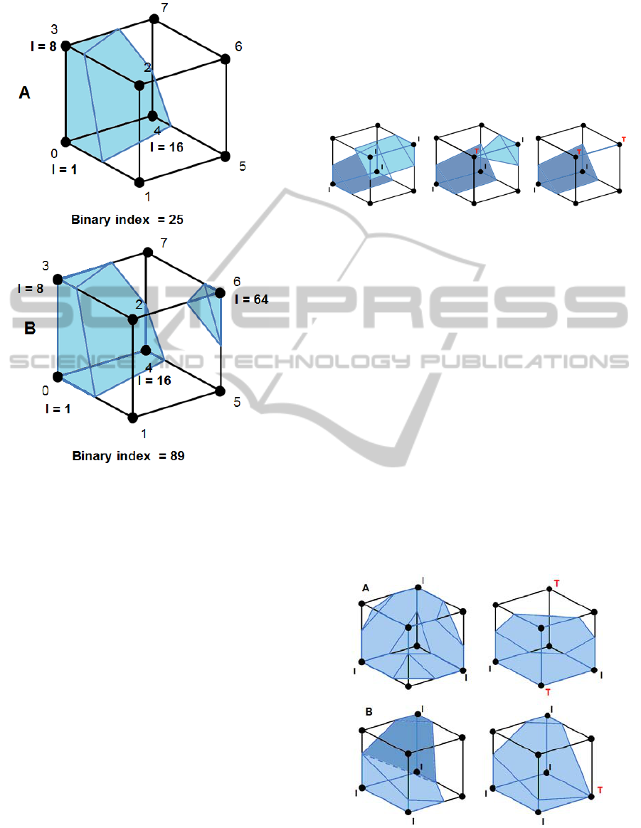
Figure 10: Example of the binary point method. Element
A is legal; 25 is in the legal element index. Element B is
illegal; 89 is not in the legal element index.
identification are shown in Figure 10 applied to a
legal element (A) and an illegal element (B).
As well as having the advantage of being simple
the method is also computationally inexpensive.
This is an important characteristic as the binary
index method is used to check element legality at
every iteration of optimization.
3.2 Further Issues in 3D Elements
After an optimization step to update the structural
boundaries and the illegal elements are identified
using the binary index method the boundaries must
be modified to eliminate the illegal elements. This
step moves the boundaries in illegal elements such
that there is only one surface cut through the
element. This is implemented by changing the status
of nodes to T-nodes, which follow the same rules in
3D as in 2D. However there are several cases that
are unique to 3D geometry.
Firstly in 2D all the illegal elements could be
fixed by changing one node to a T-node. However
this is not the case in 3D. Figure 11 shows a case
where two nodes need to be changed to T-nodes to
remove one of the cuts. Investigation has shown that
the maximum number of node changes required to
correct any illegal element cut is two, including an
element cut four times and the Impossible 4 as
shown in Figure 12.
Figure 11: Cases where changing one node to a T-node
does not make the element legal. Two neighbouring nodes
must be changed.
The second issue is that unlike 2D modelling,
changing the node closest to the boundary to a T-
node does not guarantee the smallest shift in the
boundary. In Figure 13 the change that will produce
a legal element with the smallest movement of the
boundary is to change node A to a T-node and
remove the pyramid of material around it. However
changing the node closest to the boundary would
change node B which would not make the element
legal. A more robust method of node selection is
required in 3D.
Finally changing a node to a T-node can result in
an illegal neighbouring element that shares the node.
In Figure 14 changing node X to a T-node makes
element A legal but it causes the neighbouring
element B to become illegal. To prevent this it is
necessary to check that changing a node to a T-node
does not make neighbouring elements illegal.
Figure 12: Illustration of how only one or two T-nodes are
required to eliminate an illegal cut even when the element
is cut four times as in case A. One node is required to be
changed to a T-node make an Impossible 4 legal in case B.
ALGORITHM TO MAINTAIN LINEAR ELEMENT IN 3D LEVEL SET TOPOLOGY OPTIMIZATION
345
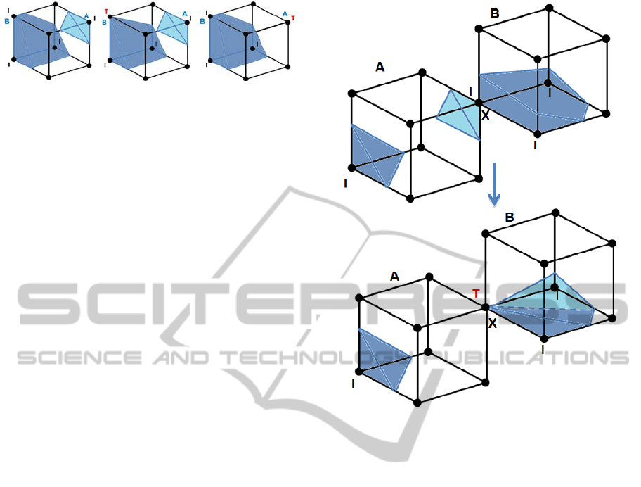
Figure 13: In this case changing the node closest the
boundary (node B) to a T-node does not make the element
legal. The least significant change to make the element
legal is to change node A to a T-node.
3.3 Fractured Elements
Due to the need to maintain legality in neighbouring
elements during the boundary modification
procedure in 3D it is possible that a simple change
of nodes of an illegal element to T-nodes is not
sufficient in eliminating all illegal elements. This
problem occurs in regions where there are multiple
structural boundaries close together. As a result
moving a boundary cut out of one element results in
an extra boundary cut appearing in neighbouring
elements. This suggests that the local structure is
porous, formed from struts that are narrower than an
element and/or islands of disconnected material.
Finite element analysis results in porous local
structures described by just a few disconnected
elements have poor accuracy and such structures are
usually a product of numerical instability such as
chequerboard patterns well-known in topology
optimization. We therefore, consider elements in
such local porous regions to be “fractured” where all
nodes in the elements are changed to T-nodes. With
no I-nodes left a fractured element is considered to
be outside the structure and hence makes no
contribution to its stiffness.
It is worth noting that fractured elements are not
a common occurrence in topology optimization;
none occur during either of the example models
shown in Figure 16 or Figure 18. If a model
produces many fractured elements, it means the
mesh is too coarse to further optimize the structure
and the mesh should be refined.
3.4 Boundary Update Algorithm for 3D
Level Set Topology Optimization
Having considered all cases for identifying and
eliminating illegal elements in 3D the following
algorithm is formulated for level set topology
optimization. This algorithm follows the usual level
set topology optimization boundary update to
eliminate illegal elements. A flow chart of this
method can be seen in Figure 15.
The first step is to identify the elements that the
Figure 14: An example when making element A legal by
changing node X into a T-node consequently makes
element B illegal.
boundary passes through by examining the node
statuses of each element. If an element contains at
least one I-node and one O-node then it is cut by a
boundary; if it has no I-nodes it is entirely outside
the structure; otherwise it is entirely inside the
structure. If an element is cut by a boundary its
legality is checked using the binary indexing method
described in Section 3.1, if the element is illegal then
it is added to the correction set. Only once the
legality of all the elements has been established does
the correction procedure begin.
For each of the elements in the correction set, the
algorithm searches for the correction that would
make the elements legal and minimize the necessary
boundary modification. The algorithm begins by
changing the status of one node only. Each node in
turn is temporarily changed to a T-node and the
binary index method is used to check if the change
has made the element legal. If so the legality of the
neighbouring elements that share the node and are
currently legal is checked to make sure the change
has not made any of these elements illegal. If all the
legal neighbouring elements remain legal then this
modification is considered a potential solution. If
there is more than one possible solution, the
ICPRAM 2012 - International Conference on Pattern Recognition Applications and Methods
346
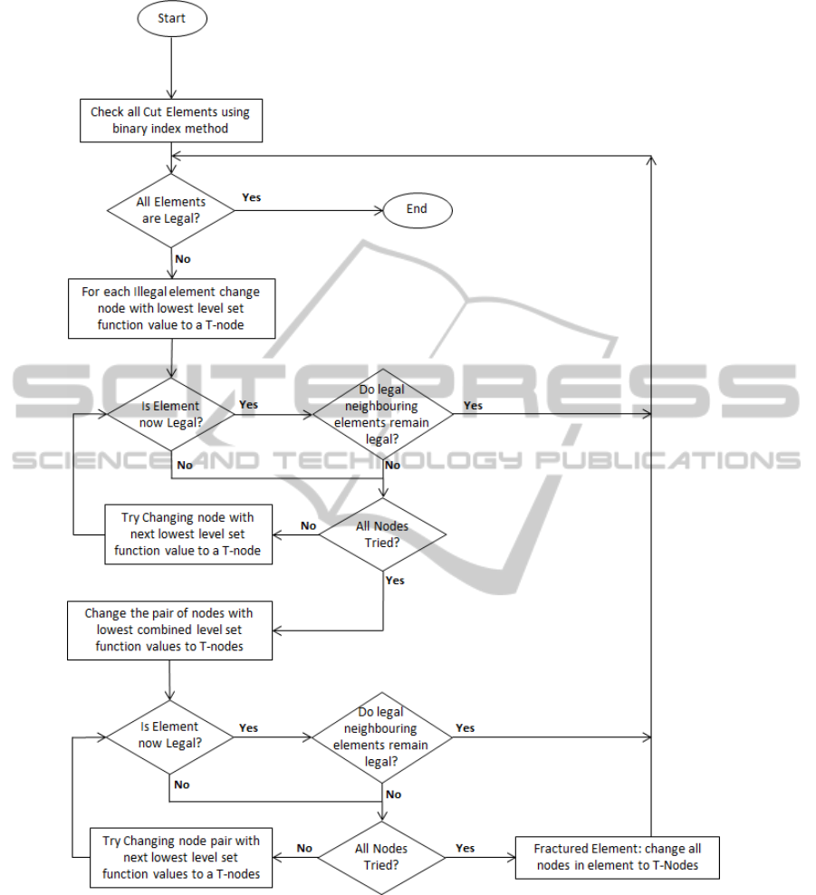
Figure 15: Flow chart for boundary correction algorithm.
one with the smallest level set function value (thus
closest to the boundary) is selected and turned into a
T-node to make the minimal change to the optimum
boundary.
If there are no possible solutions from simply
changing a single node to a T-node, a pair of nodes
is temporarily changed to T-nodes to find a two-
node solution. Again, of all the possible two-node
solutions, the lowest combined level set function
value is selected to be turned into T-nodes to make
the element legal.
In the rare situation that no suitable correction is
found changing either one or two nodes to T-nodes
then the element is considered to be fractured as
described in Section 3.3. All its nodes are turned into
T-nodes removing it from the structure. All the
neighbouring elements are then examined, to
investigate if this modification made the
ALGORITHM TO MAINTAIN LINEAR ELEMENT IN 3D LEVEL SET TOPOLOGY OPTIMIZATION
347
neighbouring elements illegal. All the new illegal
elements are then added to the correction set.
Once all illegal elements are considered and the
correction set is empty, the new solution is checked
for convergence and the optimization procedure
continues.
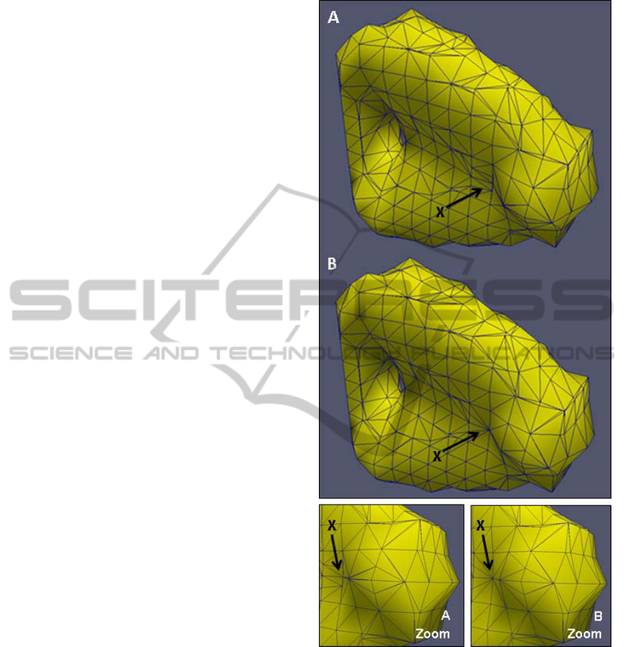
An example of the effect this algorithm can have
on the topological solution is shown in Figure 16. As
in 2D modelling a reasonable mesh density is
required to minimize the effect of this process on the
optimal boundary.
4 NUMERICAL RESULTS
The boundary update algorithm described in Section
3 ensures that there is always sufficient nodal
information to perform sensitivity computation
allowing the optimization process to reliably
proceed. This section illustrates the numerical
examples of the topology optimization.
Figure 17 shows level set topology optimization
of a 2D cantilever beam with aspect ratio 2. The
structure displays features that would be expected in
the optimum solution which is well-known (Michell,
1904). The thick beam is positioned at the top and
bottom of the design space to resist the bending of
the structure. In the centre where less bending is
strain is experienced smaller diagonal struts are
formed to provide support for the exterior structure.
A similar cantilever beam of aspect ratio 2 is
created in 3D on a course 61x30x10 mesh with a
central load downwards, as shown in Figure 18.
Figure 18 B to D shows how the structure develops
during the optimization procedure. Starting from
fully-populated continuum (B) the boundary moves
towards the optimum topology by removing material
in the centre of the beam first; leaving more material
at the top and bottom of the structure to maintain a
higher second moment of area and reduce bending.
The converged topology adopts similar features to
the 2D solution with thick beams around the outside
of the structure supported in the centre by a thinner
“web” made of multiple struts, similar to an I-beam.
5 CONCLUSIONS
During level set topology optimization it is possible
for the boundary of the structure to move in a
manner that cuts an element more than once. This
violates the modelling assumptions for 1
st
order
bilinear elements which cannot accurately represent
Figure 16: Example of how the treatment of illegal
elements affects the global structure. A shows the
structure before the element correction process. Arrow X
points to a sharp indent in the structure which cuts two
elements illegally. The correction procedure changes 4
nodes attached to these elements to T-nodes to make both
elements legal. The movement of the boundary flattens the
indent as can be seen in B; however this shift is small and
does not have a significant effect on the global topological
solution. (Note: the triangular surface mesh in these
images represents the mesh for visualization and is not
used for analysis or optimization. It is shown to highlight
the structural details.)
ICPRAM 2012 - International Conference on Pattern Recognition Applications and Methods
348
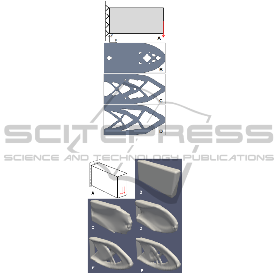
Figure 17: An Example of level set topology optimization applied to a simple cantilever beam in 2D. The modelled
situation is show in A with the development of the optimal structure is shown in images B to D.
Figure 18: Example of 3D level set topology optimization applied to a simple cantilever beam on a 61x30x10 mesh. A
shows the modelling situation and B to F show stages of the structure development from the initial continuum structure to
the final optimal structure.
two boundaries in one element. Such element cuts
are considered illegal. This paper presented a
method to make illegal element cuts legal during
level set topology optimization.
A binary index method is used to efficiently and
reliably detect illegal elements. The algorithm then
identifies the extra boundary, or boundaries, closest
to the edge of the elements and moves it outside the
element to make the element legal. The possibility of
this movement making a neighbouring element
illegal is considered by the algorithm and prevented.
Even with a relatively coarse mesh density this
method does not have a significant effect on the
global solution and produces the optimum topology.
The implementation of this method allows the
use of a regular grid of first order bilinear elements
on the geometric boundary of nodal sensitivity based
level set topology optimization. The successful
optimum solutions in 2D and 3D numerical
examples demonstrate the methods reliability and
suitability for level set topology optimization.
Possible extensions include the interface between
two materials in composite structures and contact
modelling between two surfaces. This will be
ALGORITHM TO MAINTAIN LINEAR ELEMENT IN 3D LEVEL SET TOPOLOGY OPTIMIZATION
349

investigated in future works.
REFERENCES
Allaire G., Jouve F., Toader AM., 2004. Structural
optimization using sensitivity analysis and a level-set
method. Journal of Computational Physics; 194(1):
363-393.
Dunning P D., Kim H A., 2011. Investigation and
improvement of sensitivity computation using the
area-fraction weighted fixed grid FEM and structural
optimization. Finite Elements in Analysis and Design;
47: 933-941.
Jang G., Kim Y Y., 2005. Sensitivity analysis for fixed-
grid shape optimization by using oblique boundary
curve approximation. International Journal of Solids
and Structures; 42: 3591-3609.
Wang S Y., Lim K Y., Khoo B C., Wang M Y., 2007, An
extended level set method for shape and topology
optimization. Journal of Computational Physics; 221:
395-421.
Wang S., Wang M Y., 2006, A moving superimposed
finite element method for structural topology
optimization. International Journal for Numerical
Methods in Engineering; 65:1892-1922.
Challis V J., 2010, A discrete level-set topology
optimization code written in Matlab. Structural and
Multidisciplinary Optimization; 41(3): 453-464.
Belytschko T., Parimi C., Moës N., Sukumar N., Usui S.,
2003, Structured extended finite element methods for
solids defined by implicit surfaces. International
Journal for Numerical Methods in Engineering; 56;
609-635.
Wei P., Wang M Y., Xing X., 2010, A study on X-FEM in
continuum structural optimization using a level set
model. Computer-Aided Design; 42: 708-719.
Bourke P., 1994. Polygonising a Scalar Field. http://
paulbourke.net
Michell A. G. M., 1904. The limits of economy of
material in frame-structures; Royal Society
Philosophical Magazine; 8: 589–597
ICPRAM 2012 - International Conference on Pattern Recognition Applications and Methods
350
