IMAGE SEQUENCE SUPER-RESOLUTION BASED ON LEARNING
USING FEATURE DESCRIPTORS
Ana Carolina Correia R
´
ezio, William Robson Schwartz and Helio Pedrini
Institute of Computing, University of Campinas, SP, 13083-852 Campinas, Brazil
Keywords:
Super-resolution, Machine Learning, Feature Descriptors, Image Resolution.
Abstract:
There is currently a growing demand for high-resolution images and videos in several domains of knowledge,
such as surveillance, remote sensing, medicine, industrial automation, microscopy, among others. High res-
olution images provide details that are important to tasks of analysis and visualization of data present in the
images. However, due to the cost of high precision sensors and the limitations that exist for reducing the size
of the image pixels in the sensor itself, high-resolution images have been acquired from super-resolution meth-
ods. This work proposes a method for super-resolving a sequence of images from the compensation residual
learned by the features extracted in the residual image and the training set. The results are compared with
some methods available in the literature. Quantitative and qualitative measures are used to compare the results
obtained with super-resolution techniques considered in the experiments.
1 INTRODUCTION
The resolution of a digital image is directly related
to its quality. This resolution refers to the level of
detail of its visual representation, that is, the higher
the resolution, the greater its precision to represent it
in relation to the actual image (Chaudhuri, 2001a).
In many applications, an image or a sequence of
images presents poor quality due to several physical
limitations of the sensors, such as low spatial resolu-
tion, optical distortions, noise, and limited dynamic
range (Bascle et al., 1996). In general, these degrada-
tions seriously undermine the process of image analy-
sis. In surveillance systems, for example, images cap-
tured from low cost cameras may hinder the recogni-
tion of individuals or the identification of a vehicle li-
cense plate at a certain scene (Lin et al., 2005). In ad-
dition, a person or an object usually occupies a small
region in the field of camera view, such that the por-
tion of pixels of interest in the image is usually very
small.
In several fields of knowledge, such as medicine,
biology, geology, industrial automation, surveillance,
remote sensing, among others, there is a great demand
for high-resolution images (Chaudhuri, 2001b; Patti
and Altunbasak, 2001).
Due to factors associated with cost and limitations
of acquisition devices, an alternative is to increase
the resolution and improve the psicovisual quality of
the images by applying super-resolution techniques.
Some images can suffer from a process of degradati-
on of its quality (low resolution images) due to some
factors, such as lens aberration, incorrect focus, sen-
sor displacement during acquisition, object displace-
ment, lack or excess of lighting (Bascle et al., 1996).
Super-resolution techniques have received much
attention in recent years (Liu et al., 2008; Lucien,
1999; Lin et al., 2005; Sun et al., 2008; Baker and
Kanade, 2002), whose main objective is to increase
the spatial resolution of images, removing distortions
in the acquisition, highlighting details, such as bor-
ders, or recovering important information from the set
of images.
Super-resolution techniques can be applied to a
single image, a sequence of multiple images, or
videos. Super-resolution methods for a single im-
age aim at increasing the image resolution from the
enhancement of its most relevant information, with-
out introducing blurring. Figure 1 illustrates im-
ages at low and high resolution. Super-resolution
methods for multiple images seek to create an im-
age with higher resolution from fusion information
present in multiple low resolution images. Super-
resolution methods for videos aim at generating a
high-resolution video from low-resolution frames.
The development of techniques for increasing the
sharpness of image details becomes important, since
they can improve subsequent steps of data analysis
and interpretation.
This paper presents a learning-based method for
generating high resolution images from correspond-
ing versions of the images at low-resolution. Unlike
135
Carolina Correia Rézio A., Robson Schwartz W. and Pedrini H..
IMAGE SEQUENCE SUPER-RESOLUTION BASED ON LEARNING USING FEATURE DESCRIPTORS.
DOI: 10.5220/0003861701350144
In Proceedings of the International Conference on Computer Vision Theory and Applications (VISAPP-2012), pages 135-144
ISBN: 978-989-8565-03-7
Copyright
c
 2012 SCITEPRESS (Science and Technology Publications, Lda.)

Figure 1: Examples of images (a) at low resolution and (b)
at high resolution. Images extracted from (Sun et al., 2010).
the technique developed by Yu et al. (Yu et al., 2008),
this work presents a methodology for super-resolution
also based on locally linear embedding (LLE) and
residual compensation, however, the representation of
the residual is carried out by means of feature descrip-
tors, which allows a better estimation of the super-
resolved images and avoids various artifacts. Addi-
tionally, the proposed method applies a more robust
technique for estimating the initial super-resolved im-
age than that used by Yu et al. (Yu et al., 2008),
called prior gradient profile (GPP) (Sun et al., 2010),
which has a greater focus on edge preservation. The
method is proposed for super-resolving multiple low-
resolution images, instead of only a single image, on
a high resolution image.
For extraction of feature descriptors, the
method uses the histogram of shearlet coeffi-
cients (HSC) (Schwartz et al., 2011). The HSC is
based on an accurate multi-scale analysis provided
by the shearlet transform and the use of histograms
for estimating the distribution of edge orientation.
Experimental results show that the description of the
residual using HSC provides a significant reduction
of artifacts resulting from the application of super-
resolution. The effectiveness of the proposed method
is assessed by quantitative and qualitative measures.
This paper is organized as follows. Section 2
describes some important concepts and related work
on super-resolution. Section 3 presents the proposed
super-resolution method applied to a sequence of im-
ages. Experimental results are shown and discussed
in Section 4. Finally, Section 5 concludes the paper
with final remarks.
2 RELATED WORK
Spatial resolution is associated with the size of the
smallest details visible in the image. The smaller the
sampling interval among the image points, that is, the
higher the density of points in the image, the higher
the spatial resolution of the image. This does not
mean that an image containing a large number of pix-
els necessarily has higher spatial resolution than one
with fewer pixels.
Several super-resolution methods have been pro-
posed in the literature for improving the spatial res-
olution of the images. The main objective of these
methods is to estimate a high-resolution (HR) image
from one or more low resolution (LR) images in order
to highlight details, without the addition of artifacts in
the resulting image.
The main approaches found in the literature can be
classified into three categories: methods based on de-
tail enhancement, reconstruction-based methods and
learning-based methods. These approaches are de-
scribed below.
2.1 Methods based on Detail
Enhancement
In methods based on detail enhancement, the estima-
tion of pixel values in the high resolution image is
performed by interpolating the intensity or color of
the pixels already present in the input image. After-
wards, a process is applied to reduce artifacts included
in the interpolated images.
There are several interpolation methods in the lit-
erature (Gonzalez and Woods, 2007; Lucien et al.,
1997), such that the most commonly used are the
nearest neighbor, bilinear and bicubic interpolation.
In the nearest neighbor interpolation, the orig-
inal pixel value f (x, y) is assigned to the nearest
pixel f
0
(x
0
, y
0
) in the resampled image. Although the
method is simple and has low computational cost, its
main disadvantages are the generation of distortion in
fine details and creation of jagged edges in the image.
The bilinear interpolation calculates the intensity
of each pixel value f
0
(x
0
, y
0
) by the weighted average
of four pixels adjacent away from the nearest neigh-
bors. The resulting image presents smoothing at the
edges and phase distortion, resulting in image blur-
ring.
Bicubic interpolation seeks to obtain a smooth es-
timate of the gray level or color at each pixel f
0
(x, y)
from a larger number of neighboring points of the
original image, which form a polynomial of low de-
gree. Fine details are preserved, edges are smoothed
and distortions are minimized in the resulting image.
VISAPP 2012 - International Conference on Computer Vision Theory and Applications
136

The super-resolution method called prior gradient
profile (GPP) is a parametric distribution that de-
scribes the shape and sharpness of gradient profiles
in natural images. One of the observations presented
by Sun et al. (Sun et al., 2008; Sun et al., 2010) is
that the statistical form of these profiles is stable and
invariant to the resolution of the image. From this in-
formation, a statistical relation of the image gradient
sharpness can be learned between HR and LR images.
Using the learned profile gradient relation, it is
possible to provide a constraint on the field gradient
of the HR image. Combining it with the constraint
reconstruction, it is possible to recover a high quality
image. The advantages of the GPP mentioned in (Sun
et al., 2008; Sun et al., 2010) include: (a) the gra-
dient profile is not a constraint of smoothness, there-
fore, the edges can be well recovered in the HR image
both at small and large scales; (b) the artifacts com-
mon in super-resolution, such as jagged edges, can be
avoided in the field gradient.
The high-resolution image in the GPP technique
can be obtained from the following equation
HR
t+1
= HR
t
− τ
∂E(HR)
∂HR
(1)
where
∂E(HR)
∂HR
= ((HR ∗ G) ↓ − LR) ↑ ∗ G −
β(∇
2
HR − ∇
2
HR
T
), ∇
2
HR
T
(x) = r(d(x, x
0
))∇
2
LR
u
,
G represents the Gaussian filter, ∗ is the convolution
operator, ↓ is the down-sampling operator, ∇
2
HR
T
represents the image field gradient of the HR image,
∇
2
LR
u
represents the field gradient of the LR im-
age, and ↑ is the up-sampling operator. Term ∇
2
HR
T
transforms the observed field gradient into the target
field gradient by mapping the shape and sharpness
profile of the observed gradient.
2.2 Methods based on Reconstruction
Reconstruction-based methods consist in the synthe-
sis of a single high resolution image from a sequence
of low-resolution images (Borman and Stevenson,
1998). In these methods, it is assumed that the cap-
tured images of low resolution (LR) are very sim-
ilar to each other. There are few details that set
them apart, allowing the generation of new informa-
tion to recover the image details in high resolution
(HR) (Patti and Altunbasak, 2001).
These methods recover details of sequences and
add them to the estimated high-resolution image.
Usually, they have three different phases: i) reg-
istration of the images, ii) generation of the high-
resolution grid, where their values are interpolated
from the recorded images, iii) removal of noise (Park
et al., 2003).
Irani and Peleg (Irani and Peleg, 1991) developed
a technique called iterative back-projection (IBP),
similar to the method of back-projection developed
for reconstruction of tomographic images. Each low-
resolution pixel is modeled as the projection of a
given region in the high resolution image that will
be estimated. The process starts with a first estimate
of the high resolution to simulate the low-resolution
images. Iteratively, information is added to this esti-
mated image, from a new gradient image, based on
the error between the simulated images and the ob-
served images. This gradient image is the sum of all
errors between the low resolution image and the high-
resolution image estimated by the transformation pro-
cess given by the motion estimation between the low-
resolution images. The method uses an iterative pro-
cedure to minimize the error between the original data
and the output of the model.
Projection onto convex sets (POCS) (Stark, 1988)
uses the low resolution image to produce a new image
through subpixel displacements in rows and columns.
The displacement aims at minimizing the effects of
aliasing and allowing the retrieval of new information
for the high resolution image.
The POCS method seeks to solve the problem
from a priori information described in the form of
convex sets of constraints. The search for this solution
consists of finding a value that belongs to the inter-
section of the sets. This is an iterative method, which
produces, for a finite number of steps, intermediate
solutions. The iteration ends when convergence oc-
curs or the process is interrupted by a predetermined
criterion.
Some improvements in reconstruction methods
based on POCS were developed by Patti and Altun-
basak (Patti and Altunbasak, 2001). First, the dis-
cretization of the model of continuous image forma-
tion is enhanced to allow the use of high-order in-
terpolation methods. Second, the constraint sets are
modified to reduce the number of edges present in the
estimated high resolution image.
Reconstruction by super-resolution produces an
image or a set of high resolution images from a set
of low-resolution images. In the last two decades,
several super-resolution methods have been proposed,
some of them presented in (Borman and Stevenson,
1998; Farsiu et al., 2004a). These methods are often
very sensitive to noise and to their data model, which
limits their usefulness. In (Farsiu et al., 2004b), an
alternative approach was proposed using minimiza-
tion standards and robust regularization before deal-
ing with different data models and noise.
IMAGE SEQUENCE SUPER-RESOLUTION BASED ON LEARNING USING FEATURE DESCRIPTORS
137

2.3 Methods based on Learning
In super-resolution methods based on learning, the
main objective is to estimate information, which is
not present in the original low-resolution image, from
a set of training samples.
The method proposed by Yu et al. (Yu et al., 2008)
for super-resolution of face images uses projection
onto convex sets (POCS) and residual compensation.
First, the original high resolution image is estimated
by POCS and then the residual compensation is per-
formed. The high frequency information in the im-
age is reconstructed from the learning between the
two training data sets of corresponding low and high
resolution residual images. The super-resolution im-
age is generated from the sum between the initially
estimated image and the image reconstructed by the
weights of learned residuals. The method uses a ma-
chine learning algorithm called locally linear embed-
ding (LLE) (Chang et al., 2004).
First, the method reconstructs the high resolu-
tion image initially estimated by POCS, similar to
the original high resolution image. Afterwards, it es-
timates the residual compensation and the high fre-
quency information is reconstructed by learning be-
tween the correspondence of sets of high and low res-
olution residual images. Assuming a set of N vectors
of dimension D (Yu et al., 2008), then
x = [x
1
, x
2
, ..., x
i
, ..., x
N
] (2)
For a new vector x
0
, the Euclidean distance d
i
be-
tween all other vectors x is calculated as
d
i
=
q
(x
0
− x
i
)
T
(x
0
− x
i
) (3)
The K nearest neighbors of x
0
are defined by the
Euclidean distance and, therefore, the best weights
w to rebuild x
0
from K neighbors are determined
(w = [w
1
, w
2
, ..., w
i
, ..., w
N
]), where w
i
represents the
contribution of x
i
for x
0
reconstruction. If x
i
is not be-
tween the K nearest neighbors of x
0
, then w
i
= 0, else
0 < w
i
< 1 and
∑
i
w
i
= 1.
The optimal weight w
i
is estimated using the least
squares algorithm
w
i
=
∑
j
P
i, j
∑
i
∑
j
P
i, j
(4)
where P = G
−1
and G is the covariance matrix defined
as
G
i, j
= (x
0
− x
i
)
T
(x
0
− x
i
) (5)
Since G is a singular matrix, that is, it has no in-
verse, the optimal solution can not be found by Equa-
tion 5. A relatively simple solution is to assign a small
value of α to the diagonal of G
G = G + α × I (6)
where I is a unit matrix.
The learning method proposed in (Yu et al., 2008)
considers an initial low resolution image g obtained
by degrading f (g = H f ) and an initial estimate of
super-resolution
ˆ
f obtained by the POCS method.
From the known degrading model H, the low reso-
lution residual is calculated as
ˆg = H
ˆ
f r = g − ˆg (7)
Using the LLE algorithm to learn the weights of
the reconstruction from the low-resolution residual
r and the set of residual images, the method recon-
structs the high-resolution residual ˆs from the cal-
culated weights and the corresponding data at high
resolution. From the high-resolution residual, super-
resolution image
ˆ
f
n+1
is obtained by
ˆ
f
n+1
=
ˆ
f
n
+ α ˆs ∈ (0, 1] (8)
3 PROPOSED METHOD
According to the previous section, there are
three main approaches to enhancing image res-
olutions: methods based on detail enhancement,
reconstruction-based methods and learning-based
methods. The method proposed in this work is based
on learning, in which training samples are used to es-
timate the information regarding details that are not
present in the lower resolution images. This super-
resolution technique has been inspired by (Yu et al.,
2008), which employs residual compensation.
The method developed in this work considers a
sequence of low resolution images that will be com-
bined into a single higher resolution image.
The training set, which is sampled from the se-
quence being processed due to high similarity among
the samples, needs to be pre-processed prior to the
execution, as shown in Figure 2.
Image samples in the training set are considered as
to be the high resolution (HR). These images will be
smoothed and downsampled to obtain low resolution
(LR) images. The LR images have their resolution in-
creased, generating images called SR, which will be
smoothed and downsampled to generate the images
LR
0
. The low resolution residuals are estimated by
the difference between LR and LR
0
, which the cor-
responding high resolution residuals are estimated by
the difference between images HR and SR. Feature
extraction is performed for each low resolution resid-
uals, resulting on a feature vector.
After the pre-processing, the proposed super-
resolution method for multiple images is executed, ac-
cording to the steps shown in Figure 3. This process
is described in the following paragraphs.
VISAPP 2012 - International Conference on Computer Vision Theory and Applications
138

Figure 2: Pre-processing of the training set sampled from the image sequence.
Figure 3: Data flow of the proposed method.
The execution process starts with the original se-
quence, denoted HR. This sequence is smoothed and
then downsampled, which will generate a new se-
quence called LR. The proposed method will be ap-
plied to this sequence. This is necessary so that the
original sequence can be used as a reference to assess
the results achieved.
The second step consists of increasing the resolu-
tion of the sequence LR, generating a new sequence,
called SR, with the same resolution as the original se-
quence. Then, the images are fused in pairs, in which
one of them is the first images of the sequence (refer-
ence image), as shown in Figure 4.
The process starts with N images. After the fu-
sion, the result consists of N = N − 1 images. If
the sequence size N becomes equal to 1, the result-
ing super-resolved image has been obtained and the
process is stopped. Otherwise, the resulting sequence
IMAGE SEQUENCE SUPER-RESOLUTION BASED ON LEARNING USING FEATURE DESCRIPTORS
139

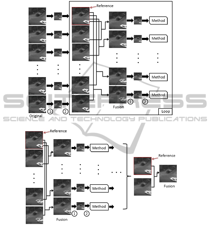
(a) Proposed method.
(b) Iterative process.
Figure 4: Proposed super-resolution method for a sequence of images.
is smoothed and downsampled, generating a new se-
quence LR
0
, in which the super-resolution for each
image will be obtained by applying the procedure de-
scribed in Section 3.1. This fusion process is illus-
trated in Figure 4(b) and Algorithm 17 presents the
main steps of the method described during this sec-
tion.
3.1 Super-resolution for Single Images
The procedure to perform super-resolution for a sin-
gle image is depicted in Figure 5. It starts by resam-
pling the low resolution image (LR) to the desired size
using a standard interpolation method such as bicu-
bic, bilinear or nearest-neighbor, or another super-
resolution method from the literature, such as GPP,
POCS or IBP (described in Section 2). This results in
VISAPP 2012 - International Conference on Computer Vision Theory and Applications
140

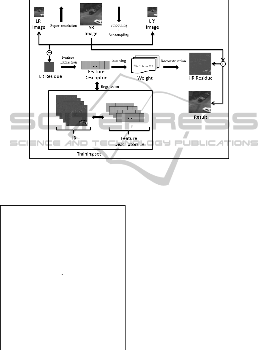
Figure 5: Super-resolution for single images.
an initial estimation of the super-resolved image, de-
noted SR.
Require: img: original image sequence, n: number
of images on this sequence, zoom: zoom factor.
Ensure: listSR: resulting image.
1: for all i = 2 to n do
2: listImg
i−1
= fusion(downsample(img
1
, zoom),
downsample(img
i
,zoom))
3: end for
4: n ← n − 1
5: while n > 1 do
6: for all i = 1 to num elements(listImg) do
7: test = smooth(listImg
i
)
8: test = downsample(teste, 1/zoom)
9: listSR
i
= singleImage(test)
10: end for
11: for all i = 2 to n do
12: listAux
i−1
= fusion(listSR
1
, listSR
i
)
13: end for
14: listImg = listAux
15: n ← n − 1
16: end while
17: return listSR
Algorithm 1: Image sequence super-resolution method.
If the initial estimation SR satisfies a similar-
ity threshold based on the root mean square error
(RMSE) between the LR and a smoothed and down-
sampled version of SR, the procedure stops. Other-
wise, the image is modified by considering the resid-
ual information. SR is added to the high resolution
residual according to Equation 9. This residual is re-
constructed by the weighted sum of several samples
belonging to the training set.
SR
n+1
= SR
n
+ α resHR (9)
To estimate the weights for the sum, features are
extracted from the low resolution residuals (resLR)
and added to a feature vector. From this vector, the
weights of k nearest-neighbors are estimated using
LLE (the k-th training samples which have the most
similar residuals to resLR). Since feature vector is as-
sociated to a low and a high-resolution sample, the
high resolution weights are used to estimate resHR in
Equation 9, where α ∈ (0, 1] denotes the importance
of the residual estimation (this parameter is experi-
mentally estimated in the next section). This process
is repeated a certain number of iterations (also esti-
mated experimentally in the next section).
IMAGE SEQUENCE SUPER-RESOLUTION BASED ON LEARNING USING FEATURE DESCRIPTORS
141

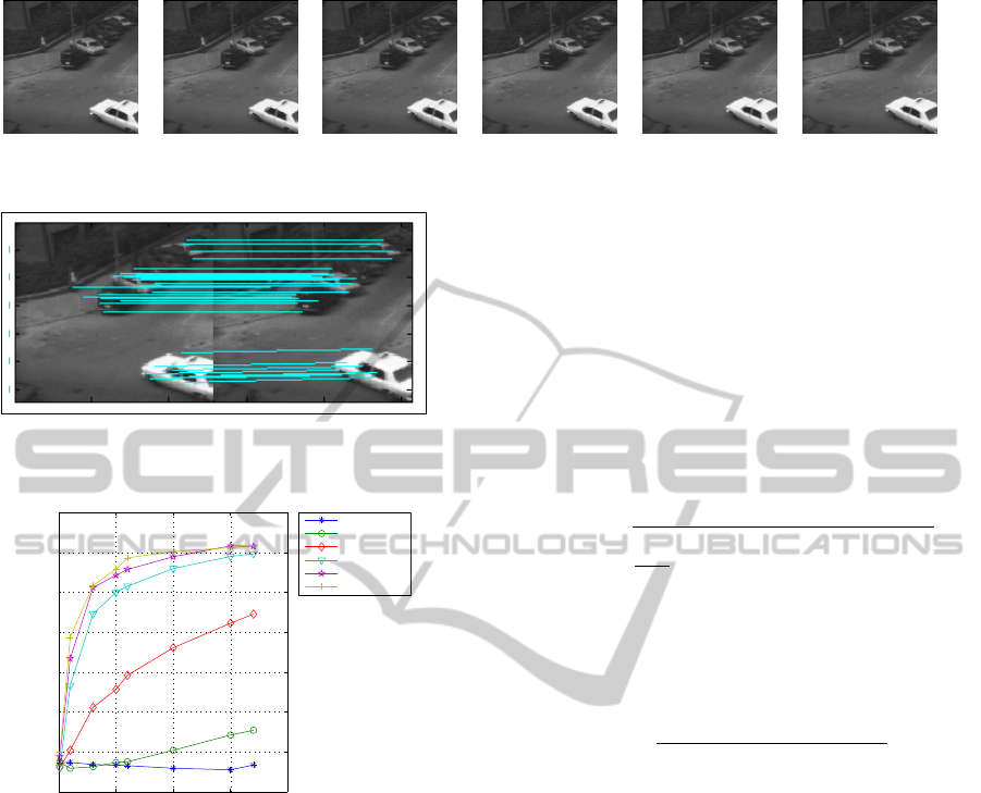
Figure 6: Examples of frames for taxi video sequence (Nagel, 2011).
Figure 7: Corresponding points between two images used
to fuse both images.
0 50 100 150 200
0
20
40
60
80
100
120
140
RMSE
Number of Iterations
alpha = 0.001
alpha = 0.01
alpha = 0.1
alpha = 0.5
alpha = 0.8
alpha = 1
Figure 8: RMSE as a function of the number of iterations
and α.
4 EXPERIMENTAL RESULTS
This section describes the experiments and compares
the results achieved by applying the proposed method.
All experiments were conducted using a Intel Core 2
Duo 2.2 GHz processor with 6GBytes of RAM on the
Windows 7 operating system.
4.1 Dataset
To evaluate the proposed method, a public access
video sequence with 41 frames was used (Nagel,
2011) (some frames are shown in Figure 6). Each
frame is in grayscale and has 256×191 pixels. In our
experiments, the frames were cropped to 128×128
pixels, since some of the compared methods work
only for square images.
4.2 Evaluation Metrics
The results obtained were assessed through the root
mean square error (RMSE) and the structural simi-
larity (SSIM), quantitative and qualitative measures,
respectively.
RMSE considers two images of equal sizes, such
that RMSE equal to 0 represents that both images are
identical. In the experiments, we consider the differ-
ence between the reference image and the resulting
super-resolved image. Equation 10 shows the RMSE,
where M and N denote the image dimensions.
RMSE =
v
u
u
t
1
MN
M−1
∑
x=0
N−1
∑
y=0
[SR(x, y) − HR(x, y)]
2
(10)
SSIM, proposed in (Wang et al., 2004), measures
the similarity between two images considering local
correlation, contrast and structures according to
SSIM(x, y) =
(2µ
x
µ
y
+C
1
)(2σxy +C
2
)
(µ
2
x
+ µ
2
y
+C
1
)(σ
2
x
σ
2
y
+C
2
)
(11)
where constants C
1
and C
2
prevent from numerical
instabilities when (µ
2
x
+ µ
2
y
) and (σ
2
x
σ
2
y
) are close to
zero. As suggested in (Wang et al., 2004), we used
C
1
= 0.01 and C
2
= 0.03. In this measure, the result-
ing values are normalized between 0 and 1, and the
closer to 1, the better the image quality.
4.3 Parameter Settings
To evaluate the proposed method, a set of parameters
has been defined in the experiments. First, the super-
resolution method used to resample the input image
to the desired size (as described in Section 3.1) was
the GPP.
In the fusion process, the images are considered in
pairs, in which one is considered as the reference im-
age. As illustrated in Figure 4(b), the reference image
corresponds to the first image of the sequence. To fuse
two images (lines 2 and 12 of Algorithm 17), the SIFT
algorithm (Lowe, 2004) was applied to detect corre-
sponding points (Figure 7). From such corresponding
points an affine transform is computed to register both
images.
VISAPP 2012 - International Conference on Computer Vision Theory and Applications
142

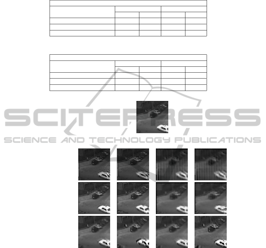
Table 1: Results achieved by the video-based super-resolution methods for a zoom factor of 2×.
Zoom factor 2×
Method 6 frames 12 frames
RMSE SSIM RMSE SSIM
IBP (Irani and Peleg, 1991) 32.5863 0.7476 34.0467 0.7081
POCS (Stark, 1988) 22.4413 0.8511 30.0020 0.7442
Proposed 10.7686 0.9604 18.0773 0.8893
Table 2: Results achieved by the video-based super-resolution methods for a zoom factor of 4×.
Zoom factor 4×
Method 6 frames 12 frames
RMSE SSIM RMSE SSIM
IBP (Irani and Peleg, 1991) 29.8295 0.7648 30.7796 0.7417
POCS (Stark, 1988) 21.5620 0.8571 29.4161 0.7501
Proposed 14.0965 0.9303 16.1489 0.9161
Original
6 frames 12 frames 6 frames 12 frames
(2×) (2×) (4×) (4×)
IBP
POCS
Proposed method
Figure 9: Results obtained for zoom factors of 2× and 4× and for sequences with 6 and 12 frames.
Finally, to achieve better results, experiments
were conducted using different setups for parameters
α (Equation 9) and the number of iterations for the
super-resolution considering single images. Accord-
ing to Figure 8, the method presents higher accuracy
for low values of α, such as 0.001. In addition to
that, the best results have been achieved with 150 it-
erations.
4.4 Results and Comparisons
Using the parameters estimated in the previous sec-
tion, the proposed method was compared to two
video-based super-resolution methods: IBP (Irani and
Peleg, 1991) and POCS (Stark, 1988) . Tables 1 and 2
show the results for zoom factors of 2× and 4× for
image sequences with 6 and 12 frames (usually, long
sequences are not considered due to the large amount
of noise inserted). These values were achieved com-
paring the super-resolved image to the reference im-
age (first image of the sequence).
Quantitative (Tables 1 and 2) and qualitative (Fig-
ure 9) results demonstrate the high accuracy of the
proposed method. According to the results shown in
Figure 9, it is also possible to see that the proposed
method presents sharper super-resolved images com-
pared to the other methods.
IMAGE SEQUENCE SUPER-RESOLUTION BASED ON LEARNING USING FEATURE DESCRIPTORS
143

5 CONCLUSIONS
Due to the increasing demand for high resolution
images and sensor limitations, super-resolution tech-
niques are fundamental tools to obtain high resolution
data.
This work proposed a super-resolution technique
based on the fusion of multiple images through resid-
ual compensation using a learning technique and
feature extraction. The comparisons performed in
our experiments showed that the proposed method
achieved higher accuracy when compared to other ap-
proaches available in the literature.
ACKNOWLEDGEMENTS
The authors are grateful to FAPESP, CAPES and
CNPq for the financial support. This research was
partially supported by FAPESP grant 2010/10618-3.
REFERENCES
Baker, S. and Kanade, T. (2002). Limits on Super-
Resolution and How to Break Them. IEEE Transac-
tions on Pattern Analysis and Machine Intelligence,
24(9):1167–1183.
Bascle, B., Blake, A., and Zisserman, A. (1996). Motion
Deblurring and Super-resolution from an Image Se-
quence. In Fourth European Conference on Computer
Vision, pages 573–582. Springer-Verlag.
Borman, S. and Stevenson, R. L. (1998). Super-Resolution
from Image Sequences - A Review. In Midwest Sym-
posium on Circuits and Systems, pages 374–378.
Chang, H., Yeung, D.-Y., and Xiong, Y. (2004). Super-
Resolution through Neighbor Embedding. In IEEE
Conference on Computer Vision and Pattern Recogni-
tion (CVPR), pages 275–282.
Chaudhuri, S. (2001a). Super-Resolution Imaging. The
Springer International Series in Engineering and
Computer Science.
Chaudhuri, S. (2001b). Super-Resolution Imaging. Kluwer
Academic Publishers.
Farsiu, S., Robinson, D., Elad, M., and Milanfar, P. (2004a).
Advances and Challenges in Super-Resolution. Inter-
national Journal of Imaging Systems and Technology,
14:47–57.
Farsiu, S., Robinson, M. D., Elad, M., and Milanfar, P.
(2004b). Fast and Robust Multiframe Super Res-
olution. IEEE Transactions on Image Processing,
13(10):1327–1344.
Gonzalez, R. and Woods, R. (2007). Digital Image Process-
ing. Prentice Hall.
Irani, M. and Peleg, S. (1991). Improving Resolution by Im-
age Registration. Graphical Models and Image Pro-
cessing, 53(3):231–239.
Lin, F. C., Fookes, C. B., Chandran, V., and Sridha-
ran, S. (2005). Investigation into Optical Flow
Super-Resolution for Surveillance Applications. In
APRS Workshop on Digital Image Computing: Pat-
tern Recognition and Imaging for Medical Applica-
tions, Brisbane, Australia.
Liu, X., Song, D., Dong, C., and Li, H. (2008). MAP-Based
Image Super-Resolution Reconstruction. In Proceed-
ings of World Academy of Science, pages 208–211.
Lowe, D. (2004). Distinctive Image Features from Scale-
Invariant Keypoints. International Journal of Com-
puter Vision, 60:91–110.
Lucien, W. (1999). Definitions and Terms of Reference in
Data Fusion. IEEE Transactions on Geosciences and
Remote Sensing, 37(3):1190–1193.
Lucien, W., Ranchin, T., and Mangolini, M. (1997). Fu-
sion of Satellite Images of Different Spatial Res-
olutions: Assessing the Quality of Resulting Im-
ages. Photogrammetric Engineering & Remote Sens-
ing, 63:691–699.
Nagel, H.-H. (2011). Image Sequence
Server. Institut f
¨
ur Algorithmen und
Kognitive Systeme, Universit
¨
at Karlsruhe.
http://i21www.ira.uka.de/image sequences/.
Park, S. C., Park, M. K., and Kang, M. G. (2003).
Super-Resolution Image Reconstruction: A Techni-
cal Overview. IEEE Signal Processing Magazine,
20(3):21–36.
Patti, A. J. and Altunbasak, Y. (2001). Artifact Reduc-
tion for Set Theoretic Super Resolution Image Recon-
struction with Edge Adaptive Constraints and Higher-
Order Interpolants. IEEE Transactions on Image Pro-
cessing, 10(1):179–186.
Schwartz, W., da Silva, R., Davis, L., and Pedrini, H.
(2011). A Novel Feature Descriptor Based on the
Shearlet Transform. In IEEE International Confer-
ence on Image Processing, Brussels, Belgium.
Stark, H. (1988). Theory of Convex Projection and its Ap-
plication to Image Restoration. IEEE International
Symposium on Circuits and Systems, pages 963–964.
Sun, J., Sun, J., Xu, Z., and Shum, H.-Y. (2008). Image
Super-resolution using gradient profile prior. IEEE
Conference on Computer Vision and Pattern Recogni-
tion.
Sun, J., Sun, J., Xu, Z., and Shum, H.-Y. (2010). Gradi-
ent Profile Prior and Its Applications in Image Super-
Resolution and Enhancement. IEEE Transactions on
Image Processing.
Wang, Z., Bovik, A., Sheikh, H., and Simoncelli, E. (2004).
Image Quality Assessment: From Error Visibility to
Structural Similarity. IEEE Transactions on Image
Processing, 13(4):600–612.
Yu, H., Xiang, M., Hua, H., and Chun, Q. (2008). Face
Image Super-Resolution through POCS and Residue
Compensation. IET Conference Publications, pages
494–497.
VISAPP 2012 - International Conference on Computer Vision Theory and Applications
144