HIGH RESOLUTION POINT CLOUD GENERATION

FROM KINECT AND HD CAMERAS USING GRAPH CUT

Suvam Patra, Brojeshwar Bhowmick, Subhashis Banerjee and Prem Kalra

Department of Computer Science and Engineering, Indian Institute of Technology Delhi, New Delhi, India

Keywords:

Kinect, Resolution Enhancement, Graph Cut, Normalized Cross Correlation, Photo Consistency, VGA, HD.

Abstract:

This paper describes a methodology for obtaining a high resolution dense point cloud using Kinect (Smisek

et al., 2011) and HD cameras. Kinect produces a VGA resolution photograph and a noisy point cloud. But

high resolution images of the same scene can easily be obtained using additional HD cameras. We combine

the information to generate a high resolution dense point cloud. First, we do a joint calibration of Kinect and

the HD cameras using traditional epipolar geometry (Hartley and Zisserman, 2004). Then we use the sparse

point cloud obtained from Kinect and the high resolution information from the HD cameras to produce a dense

point cloud in a registered frame using graph cut optimization. Experimental results show that this approach

can signiﬁcantly enhance the resolution of the Kinect point cloud.

1 INTRODUCTION

Nowadays, many applications in computer vision are

centred around generation of a complete 3D model of

an object or a scene from depth scans or images. This

traditionally required capturing images of the scene

from multiple views to generate a model of the scene.

However, today with the advent of affordable range

scanners, reconstruction of scenes from multi-modal

data which include image as well as depth scans of

objects and scenes help in more accurate modelling

of 3D scenes.

There has been considerable work with time-of-

ﬂight (ToF) cameras which capture depth scans of the

scene by measuring the travel time of an emitted IR

wave from the device reﬂected back from the object

(Schuon et al., 2008). Recently, a much cheaper range

sensor has been introduced by Microsoft called the

Kinect (Smisek et al., 2011) which has an inbuilt cam-

era, an IR emitter and a receiver. The emitter projects

a predetermined pattern whose reﬂection off the ob-

ject provides the depth cues for 3D reconstruction.

Though Kinect produces range data only in VGA res-

olution, this data can be very useful as an initial es-

timate for subsequent resolution enhancement. There

have been several approaches to enhance the resolu-

tion of a point cloud obtained from range scanners

or ToF cameras, using interpolation or graph based

techniques (Schuon et al., 2009; Schuon et al., 2008).

Diebel

et.al. (Diebel and Thrun, 2006) used a MRF based

approach whose basic assumption is that depth dis-

continuities in scene often co-occur with intensity or

brightness changes in the scene, or in other words

regions of similar intensity in a neighbourhood have

similar depth. Yang et.al. (Qingxiong Yang and Nistr,

2007) make the same assumption and use a bilateral

ﬁlter to enhance the resolution in depth. However, the

assumption is not universally true and may result in

over smoothing of the solution.

Sebastian et. al. (Schuon et al., 2009; Schuon

et al., 2008), use a super-resolution algorithm on low

resolution LIDAR ToF cameras and they rely on the

depth data for detecting depth discontinuities instead

of relying on regions of image smoothness.

In this paper we propose an algorithm for depth

super-resolution using additional information from

multiple images obtained through HD cameras. We

from Kinect with what can be obtained from the HD

cameras using multiple views geometry and carry out

a dense 3D reconstruction in the registered frame us-

ing two basic criteria: i) photo-consistency (Kutu-

lakos and Seitz, 1999) and ii) rough agreement with

Kinect. The reconstructed point cloud is at least ten

times denser in comparison to the initial point cloud.

In this process we also ﬁll up the holes of the initial

Kinect point cloud.

311

Patra S., Bhowmick B., Banerjee S. and Kalra P..

HIGH RESOLUTION POINT CLOUD GENERATION FROM KINECT AND HD CAMERAS USING GRAPH CUT.

DOI: 10.5220/0003863003110316

In Proceedings of the International Conference on Computer Vision Theory and Applications (VISAPP-2012), pages 311-316

ISBN: 978-989-8565-04-4

 2012 SCITEPRESS (Science and Technology Publications, Lda.)

2 PROPOSED METHODOLOGY

2.1 Camera Calibration

We determine the camera internal calibration matrices

(Hartley and Zisserman, 2004) for the Kinect VGA

camera and all the HD cameras ofﬂine using a state

of the art camera calibration technique (Zhang, 2000).

Henceforth we assume that all the internal camera cal-

ibration matrices are known and deﬁne the 3 ×4 cam-

era projection matrix for the Kinect VGA camera as

P = K[I|0] (1)

where K is the camera internal calibration matrix of

the Kinect VGA camera. In other words, Kinect is

our world origin.

We use ASIFT (Morel and Yu, 2009) to obtain

image point correspondences and for every HD cam-

era we compute the extrinsic camera parameters us-

ing standard epipolar geometry (Hartley and Zisser-

man, 2004). For each HD camera we ﬁrst carry out

a robust estimation of the fundamental matrix (Hart-

ley and Zisserman, 2004). Given a set of image point

correspondences x and x

, the fundamental matrix F

is given by:

Fx = 0 (2)

and can be computed using eight point correspon-

dence.

Once, the Fundamental Matrix is known, we can

estimate the external calibration from essential matrix

E, derived from Fundamental matrix using the equa-

tion as in (Hartley and Zisserman, 2004)

E = K

FK = [t]

R = R[R

where, K

is the

internal calibration matrix of the HD camera. As this

essential matrix has four possible decompositions, we

can select one of them using the cheirality check

(Hartley and Zisserman, 2004) on Kinect point cloud.

The projection matrix of the HD camera in the

Kinect reference frame is then given as

= K

[R|t] (3)

2.2 Generation of High Resolution

Point Cloud

Normalized cross correlation(NCC) method, which

tries to ﬁnd point correspondences in an image pair

by computing statistical correlation between the win-

dow centred at the candidate point, is an inadequate

tool for ﬁnding dense point correspondences. Pro-

jecting the sparse Kinect point cloud on to an HD im-

age leaves most pixels without depth labels, and one

can attempt to establish correspondence for these pix-

els using normalized cross correlation along rectiﬁed

epipolar lines. Once the correspondence is found we

can obtain the 3D point for this correspondent pair

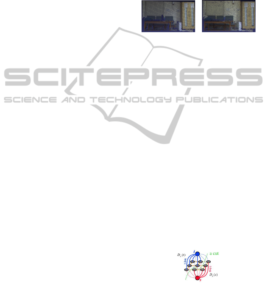
using stereo triangulation technique. In ﬁgure 1 we

show a result obtained using NCC. The reconstruc-

tion has many holes due to ambiguous cross correla-

tion results and incorrect depth labels.

(a) Initial Kinect point

cloud.

(b) High resolution point

cloud generated by NCC.

Figure 1: Resolution enhancement using NCC.

The voxel labelling problem can be represented as

one of minimizing an energy function of the form

E(L) =

∑

p∈P

) +

∑

(p,q)∈N

p,q

, Lq) (4)

where P is the set of voxels to be labelled, L =

|p ∈ P } is a 0-1 labeling of the voxel p, D

(.) is

data term measuring the consistency of the label as-

signment with the available data, N deﬁnes a neigh-

bourhood system for the voxel space and each V

p,q

(.)

is a smoothness term that measures the consistency of

labelling at neighbouring voxels.

When the above energy minimization problem

is represented in graphical form (Boykov and Kol-

mogorov, 2004), we get a two terminal graph with

one source and one sink nodes representing the two

possible labels for each voxel (see ﬁgure 2). Each

voxel is represented as a node in the graph and each

node is connected to both source and sink nodes with

edge weights deﬁned according to the data term of

the energy function. In addition, the voxel nodes are

also connected to each other with edges, with edge

strengths deﬁned according to the neighbourhood in-

teraction term. A minimum cut through this graph

gives us a minimum energy of the conﬁguration.

Figure 2: A two terminal graph from (Boykov and Kol-

mogorov, 2004).

VISAPP 2012 - International Conference on Computer Vision Theory and Applications

312

2.2.1 Assigning Cost to the Data Term

Photo consistency (Kutulakos and Seitz, 1999) is one

of the most frequently used measures for inter image

consistency. However, in real situations, several vox-

els in a close neighbourhood in depth satisfy the photo

consistency constraint resulting in a “thick” surface

as demonstrated in top view in ﬁgure 3. In view of

this, we use closeness to initial Kinect data as an ad-

ditional measure to resolve this problem of thickness

in the output high resolution point cloud.

(a) Acual view

of the scene

from front.

(b) Top

view without

distance

measure.

with distance

measure.

Figure 3: Comparison between resolution enhancement

without and with distance measure.

We deﬁne the data term based on the following

two criteria: i) Adaptive photo consistency measure

for each voxel. ii)Distance of each voxel from its

nearest approximate surface.

We use the photo consistency measure suggested

by Slabaugh et. al.(Slabaugh and Schafer, 2003). We

project each voxel i on to the N HD images and cal-

culate the following two measures:

1. S(i), the standard deviation of the intensity values

in the projection neighbourhoods calculated over

all N images.

2. ¯s(i), the average of the standard deviation in the

projection neighbourhoods for each image projec-

tion.

The voxel i is photo consistent over the N images if

the following condition is satisﬁed

S(i) < τ

+ τ

∗ ¯s(i) (5)

where τ

and τ

are global and local thresholds to be

suitably deﬁned depending on the scene. The overall

threshold speciﬁed by the the right hand side of the

above inequality changes adaptively for each voxel.

For each voxel we assign a weight D

photo

(.) for the

terminal edges in the graph based on this threshold.

photo

(i) = photocost ∗ exp(−

S(i)

+ τ

∗ ¯s(i)

) (6)

with the source and

photo

(i) = photocost ∗ (1 − exp(−

S(i)

+ τ

∗ ¯s(i)

))

(7)

with the sink

where, S(i) and τ

+ τ

∗ ¯s(i) is the standard devia-

tion and the adaptive threshold respectively for the i

voxel and photocost is a scale factor. Here the ex-

pression inside the exponential gives the normalized

standard deviation of i

voxel.

As a pre-processing step before applying graph

cut, we create an approximate surface (Alexa and

Behr, 2003) for each non-Kinect voxel using the

Kinect voxels in its neighbourhood N

of size K ×

K × K. We pre-process the Kinect point cloud to

generate an approximate surface for each non-Kinect

voxel in our voxel space in the following way:

We consider S

as the surface that can be con-

structed with the voxels P = {p

} captured by the

Kinect. Then, as suggested in (Alexa and Behr,

2003), we try to replace S

with an approximate sur-

face S

with reduced set of voxels R = {r

}. This

is done in two steps: A local reference plane H =

{x|

n, x

− D = 0, x ∈ R

}, n ∈ R

, ||n|| = 1 is con-

structed using the moving least squares ﬁt on the the

point p

under consideration. The weights for each p

is a function of the distance from the projected cur-

rent voxel on to the plane. So, H can be determined

by locally minimizing

∑

i=1

(

n, p

− D)

θ(||p

− q||) (8)

where θ is a smooth monotonically decreasing func-

tion, q is the projected point on the plane correspond-

ing to the voxel r, n is the normal and D is the per-

pendicular distance from the origin of the plane. As-

suming q = r + tn with t as a scale parameter along

the normal, equation(8) can be rewritten as

∑

i=1

(

n, p

− r −tn

)

θ(||p

− r −tn||) (9)

Let q

be the projection of p

on H and f

be the

height of p

over H. We can ﬁnd the surface estimate

Z = g(X,Y ) by minimizing the least squares equation

given by:

∑

i=1

(g(x

, y

) − f

)

θ(||p

− q||) (10)

where x

and y

are the x and y values correspond-

ing to the i

voxel and θ is a smooth monotonically

decreasing function which is deﬁned as:

θ(d) = e

−

(11)

where, h is the ﬁxed parameter which depicts the

spacing between neighbouring voxels. It reﬂects the

smoothness in the surface. For our experiment we

have taken a fourth order polynomial ﬁtting.

HIGH RESOLUTION POINT CLOUD GENERATION FROM KINECT AND HD CAMERAS USING GRAPH CUT

313

This surface is locally smooth and usually lacks

geometric details, but provides a good measure for the

approximate depth of the surface.

Hence, the second cost that we include in the data

term is based on the distance of the current voxel from

the pre-computed surface that ﬁts that voxel. So, we

project each of the non-Kinect voxel on to the pre-

computed surface (Alexa and Behr, 2003). Ideally

if the voxel is on the surface then the difference be-

tween its actual coordinates and projected coordinates

should be small, which encourage us to use this mea-

sure in the data term. Accordingly, we assign a cost

to D

on the basis of the euclidean distance between

its actual coordinates and projected coordinates on the

approximate surface.

dist

(i) =

P(r

) − r

dist threshold

(12)

with the source and

dist

(i) = 1 − D

dist

(i) (13)

with the sink. Here, the threshold dist threshold is

experimentally determined on the basis of the scene

under consideration. The total cost is expressed as:

(i) = D

dist

(i) ∗ D

photo

(i) (14)

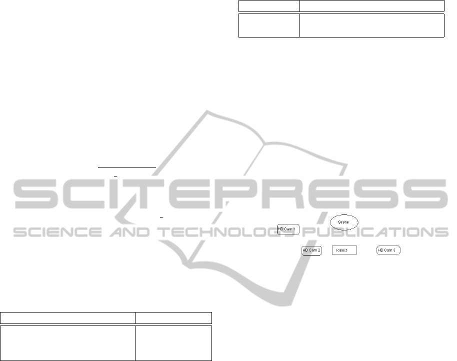
Table 1: Assignment of D

(i) Type of Voxel

∞ with source and Kinect voxel

0 with sink

Based on equation(6,7,12,13,14) Non-Kinect voxel

The cost D

(.) is assigned to a Kinect voxel so that

it is turned “ALWAYS ON”. After that, for each non-

Kinect voxel ﬁrst a distance check is done followed by

a photo consistency check over all the N HD images.

Then accordingly a cumulative cost is assigned based

on the equations above.

2.2.2 Assigning Cost to the Smoothness Term

We have assigned a constant smoothness cost to the

edges between each of the voxels and its neighbour-

hood N . Here, we have taken N to be the 6-

neighbourhood of each voxel.

Smoothness cost is assigned according to the Potts

model(Kolmogorov and Zabih, 2004; Boykov et al.,

2001). We can represent V

p,q

( f

, f

) = U

p,q

.δ( f

6= f

) (15)

Here, we have taken V

p,q

from Potts model as in Table

2. After assigning the data and smoothness costs to

the graph edges, we run the min-cut on this graph.

Table 2: Assignment of V

p,q

based on Potts model.

p,q

( f p, f q) Condition

0 f p = f q(Both are Kinect voxels)

100 Otherwise

3 RESULTS

We provide experimental results on both indoor and

outdoor scenes. For capturing the HD images we

have used the SONY HVR-Z5P camera which has an

image resolution of 1440 × 1080. This camera was

placed at multiple positions to capture images of the

same scene from different viewpoints. The experi-

mental set-up for capturing a typical scene by one

Kinect and three HD cameras has been depicted in

ﬁgure 4.

Figure 4: Our experimental set-up for capturing a typical

scene.

We have used a Dell Alienware i7 machine with

6GB RAM support for producing the results. In our

case the number of voxels that we take for the scene

depends largely on the amount of physical memory

of the machine. The ﬁgure 5 shows the resolution en-

hancement of an indoor scene done using one Kinect

and two HD cameras. Figure 5b shows the high res-

olution point cloud generated with our method. In

this all the holes have been ﬁlled up in contrast to

the point cloud generated using NCC based method

as shown in ﬁgure 1b. There are almost no outlier

points. Here we have used 300×300×100 voxels and

the value of τ

= 60 and τ

= 0.5. Figure 6 shows the

result of resolution enhancement on an outdoor scene

in the archaeological site of Hampi using one Kinect

and two HD cameras. The point cloud is at least 10

times denser than the initial point cloud. The value of

and τ

were chosen to be 80 and 0.5 respectively.

Figure 7 also shows the resolution enhancement on

another sculpture at Hampi using one Kinect and two

HD cameras. The values of τ

and τ

were similar to

ﬁgure 6.

Figure 8 shows the resolution enhancement of a

toy model where the surface is not smooth. This ex-

periment was performed using one Kinect and three

HD cameras. We have shown the dense point cloud

corresponding to both the low resolution scene as well

VISAPP 2012 - International Conference on Computer Vision Theory and Applications

314

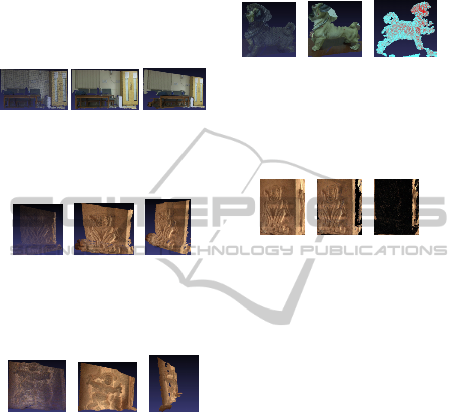
as the high resolution scene and ﬁnally overlapped

their coloured depth map to show that the geometry

is not distorted in any way. In order to do a quantita-

tive evaluation of our methods we have adopted two

approaches.

(a) Initial point

cloud.

(b) High resolu-

tion point cloud.

Figure 5: Indoor scene- A typical room. (a) Initial low

resolution point cloud from Kinect, (b) and (c) front and

side view of the high resolution point cloud generated by

our method with τ

= 80 and τ

= 0.5.

(a) Initial

point cloud.

(b) High resolu-

tion point cloud.

view.

Figure 6: Archaeological scene1- A sculpture depicting a

monkey on a pillar. (a) Initial low resolution point cloud

from Kinect, (b) and (c) front and side view of the high

resolution point cloud generated by our method with τ

60 and τ

= 0.5.

(a) Initial point

cloud.

(b) High resolu-

tion point cloud.

Figure 7: Archaeological scene2- A sculpture depicting a

goddess on a pillar. (a) Initial low resolution point cloud

from Kinect, (b) and (c)front and side view of the high res-

olution point cloud generated by our method with τ

= 60

and τ

= 0.5.

3.1 Veriﬁcation through Projection on

Another Camera

In order to demonstrate the efﬁciency of our method

we have computed the projection matrix of a different

camera which is seeing the same scene as of ﬁgure 6,

little displaced from the original cameras used for res-

olution enhancement and whose external calibration

matrix [R|t] is known beforehand. We have used this

projection matrix to project the HD point cloud onto

(a) Initial point

cloud.

(b) High res-

olution point

cloud.

maps overlapped.

Figure 8: Indoor Scene- A model of a dog. (a) Initial low

resolution point cloud from Kinect, (b) front view of the

high resolution point cloud generated by our method with

= 70 and τ

= 0.5, (c) blue HD depth map overlapped

with red low resolution depth map showing that the geome-

try is preserved.

(a) Original

image.

(b) Pro-

jected

image.

ference

image.

Figure 9: Veriﬁcation through projection on another cam-

era for the scene in ﬁgure 6. The difference image in which

around 90% is black, shows that the geometry is preserved.

a 2D image and have taken the difference between the

projected image and the ground truth. The difference

image in ﬁgure 9c is around 90% black showing that

the HD point cloud generated by our method was ge-

ometrically accurate.

3.2 Veriﬁcation through Interpolation

and Comparison

In order to show that the depth map of the HD point

cloud generated by our method conforms to the point

cloud generated by Kinect, we generated an interpo-

lated point cloud for the initial point cloud of ﬁgure

6 by ﬁtting an MLS surface of order four through it.

In order to quantify that our result show better depth

variations than the interpolated point cloud, we took

a part of each of the point clouds generated by the

interpolation method and our method; and compared

them with that of the Kinect point cloud. The stan-

dard deviation of the depth variations in the selected

part of the point cloud generated by interpolation

was 0.010068 whereas the same by our method was

0.021989, which is much closer to the standard devi-

ation generated by original point cloud i.e. 0.024674.

HIGH RESOLUTION POINT CLOUD GENERATION FROM KINECT AND HD CAMERAS USING GRAPH CUT

315

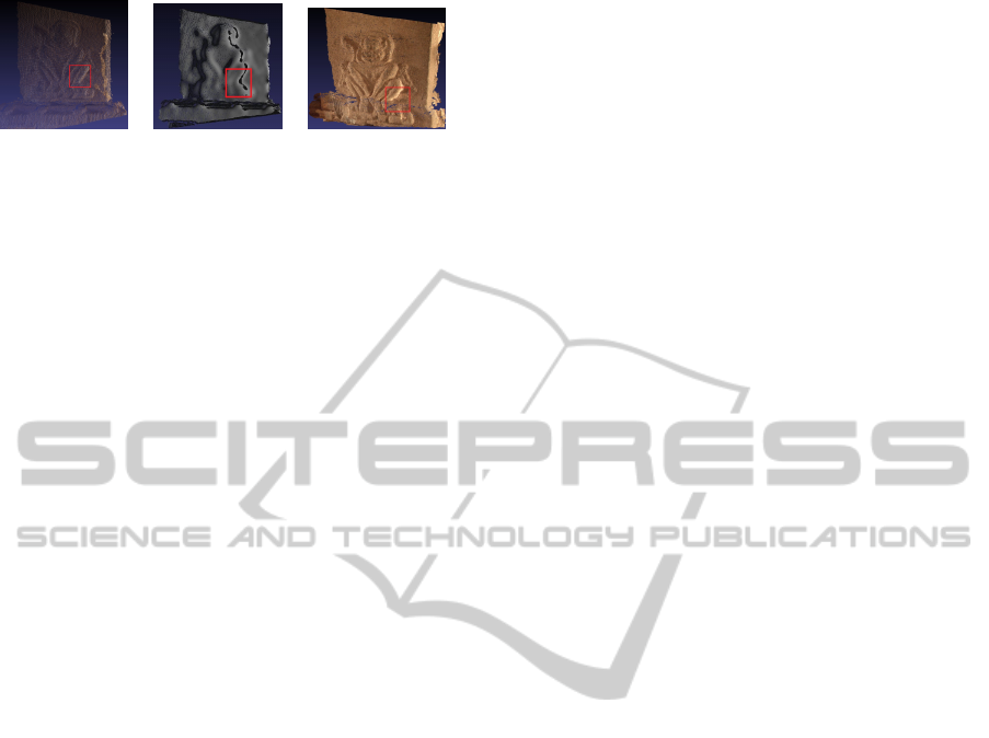
(a) Original

Kinect point

cloud.

(b) Interpolated

point cloud.

cloud generated

by our method.

Figure 10: Veriﬁcation through interpolation and compar-

ison. The area selected by the red rectangle shows the part

selected for quantitative estimation of the depth variations.

4 CONCLUSIONS

We have presented a methodology which combines

HD resolution images with the low resolution Kinect

to produce high-resolution dense point cloud using

graph cut. Firstly, Kinect and HD cameras are regis-

tered to transfer Kinect point cloud to the HD camera

for obtaining high resolution point cloud space. Then,

we discretize the point cloud in voxel space and for-

mulate a graph cut formulation which take care of the

neighbor smoothness factor. This methodology pro-

duces good high resolution image with the help of low

resolution Kinect point cloud which could be useful in

building high resolution model using Kinect.

ACKNOWLEDGEMENTS

The authors gratefully acknowledge Dr. Subodh Ku-

mar, Neeraj Kulkarni, Kinshuk Sarabhai and Shruti

Agarwal for their constant help in providing several

tools for Kinect data acquisition, module and error

notiﬁcation respectively.

Authors also acknowledge Department of Science

and Technology, India for sponsoring the project on

“Acquisition, representation, processing and display

of digital heritage sites” with number “RP02362”

under the India Digital Heritage programme which

helped us in acquiring the images at Hampi in Kar-

nataka, India.

REFERENCES

Alexa, M. and Behr, J. (2003). Computing and rendering

point set surfaces. In IEEE Transactions on Visualiza-

tion and Computer Graphics.

Boykov, Y. and Kolmogorov, V. (2004). An experimental

comparison of min-cut/max-ﬂow algorithms for en-

ergy minimization in vision. In IEEE Transactions

on Pattern Analysis and Machine Intelligence, Vol. 26,

No. 9, pages 1124–1137.

Boykov, Y., Veksler, O., and Zabih, R. (2001). Fast approx-

imate energy minimization via graph cuts. In IEEE

Transactions on Pattern Analysis and Machine Intel-

ligence, vol. 23, pages 1222–1239.

Diebel, J. and Thrun, S. (2006). An application of markov

random ﬁelds to range sensing. in advances in neural

information processing. In Advances in Neural Infor-

mation Processing Systems, page 291 298.

Hartley, R. and Zisserman, A. (2004). Multiple View Geom-

etry in Computer Vision. Cambridge University Press,

New York, 2nd edition.

Kolmogorov, V. and Zabih, R. (2004). What energy func-

tions can be minimized via graph cuts? In IEEE

Transactions on Pattern Analysis and Machine Intel-

ligence, pages 147–159.

Kutulakos, K. and Seitz, S. (1999). A theory of shape by

space carving. In 7th IEEE International Conference

on Computer Vision, volume I, page 307 314.

Morel, J.-M. and Yu, G. (2009). Asift: A new framework

for fully afﬁne invariant image comparison. In SIAM

Journal on Imaging Sciences. Volume 2 Issue 2.

Qingxiong Yang, Ruigang Yang, J. D. and Nistr, D. (2007).

Spatial-depth super resolution for range images. In

IEEE Conference on Computer Vision and Pattern

Recognition.

Schuon, S., Theobalt, C., Davis, J., and Thrun, S. (2008).

High-quality scanning using time-of-ﬂight depth su-

perresolution. In IEEE Computer Society Conference

on Computer Vision and Pattern Recognition Work-

shops.

Schuon, S., Theobalt, C., Davis, J., and Thrun, S. (2009).

Lidarboost depth superresolution for tof 3d shape

scanning. In IEEE Conference on Computer Vision

and Pattern Recognition.

Slabaugh, G. and Schafer, R. (2003). Methods for volumet-

ric reconstruction of visual scenes. In IJCV 2003.

Smisek, J., Jancosek, M., and Pajdla, T. (2011). 3d with

kinect. In IEEE Workshop on Consumer Depth Cam-

eras for Computer Vision.

Zhang, Z. (2000). A ﬂexible new technique for camera cal-

ibration. In IEEE Transactions On Pattern Analysis

And Machine Intelligence, VOL. 22, NO. 11.

VISAPP 2012 - International Conference on Computer Vision Theory and Applications

316