
ABOUT GRADIENT OPERATORS ON HYPERSPECTRAL
IMAGES
Ramón Moreno and Manuel Graña
Computational Intelligence Group, University of the Basque Country, San Sebastián, Spain
Keywords: Hyperspectral, Hyperspherical coordinates, Gradient, Chromatic Edge, Shadows.
Abstract: Gradient operators allow image segmentation based on edge information. Gradient operators based on
chromatic information may avoid apparent edges detection due to illumination effects. This paper proposes
the extension of chromatic gradients defined for RGB color images to images with n-dimensional pixels. A
spherical coordinate representation of the pixel's content provides the required chromatic information. The
paper provides results showing that gradient operators defined on the spherical coordinate representation
effectively avoid illumination induced false edge detection.
1 INTRODUCTION
Edge detection is a key step in some image
segmentation process. Edges are customarily
computed by applying linear gradient operators (i.e.
Sobel, Prewitt, Canny (Wang, 1997; Hildreth, 1987;
Gonzalez & Woods, 1992)). In color images,
gradients operators can be applied to each image
dimension independently, combining the results
afterwards. Alternatively, k-means clustering can be
applied to obtain color regions, defining the edges as
the boundaries of the found regions. The definition
of gradient operators on multi-dimensional pixel
images is an open research issue (Cheng, Jiang, Sun,
& Wang, 2001). Some approaches try to exploit the
properties of the color space (RGB, HSI, HSV, CIE
L*a*b, CIE L*u*v) to obtain sensible edge
detections. Chromatic gradient operators have been
proposed on the basis of the spherical representation
of the color points (Moreno, Graña, & Zulueta,
2010). Higher dimension images, hyperspectral
images, are becoming more common due to the
lowering cost of hyperspectral cameras, and the
growing number of airborne and satelite
hyperspectral sensors deployed by a number of
agencies. The issue of edge detection and the effect
of shadows and highlights is also open in this kind
of images. In many cases, shadows are hand
annotated in the remote sensing images to prevent
miss-segmentation. Chromaticity concepts have not
been extended to the hyperspectral image domain so
far, though they can be useful to improve
segmentation results. This paper proposes the
hyperspherical coordinate representation of the n-
dimensional Euclidean space (Moreno et al., 2010)
in order to introduce images. Hyperspherical
coordinate color representation allows to separate
chromaticy and intensity, the main colorimetrical
separation, without changing the image space. It is
therefore possible to extend Prewitt-like gradient
operators defined on the image pixels' chromaticity
(Moreno et al., 2010) to the hyperspectral case.
Those operators are independent of the image
luminosity, avoiding false edge detection on
highlights and shadows in the hyperspectral case.
This paper is outlined as follows: in Sec. 2 we
discuss about the Hyperspherical coordinates, giving
in 2.1 the transformation from Euclidean coordinates
to Hyperspherical coordinates. After that, in Sec. 3
we discuss about gradients, and in Sub-sec.3.1 we
will present a chromatic gradient operator. In Sec. 4
we will show the experimental results, finishing this
work in Sec. 5 with the conclusions.
2 HYPERSPHERICAL
COORDINATES AND
CHROMATICITY
An n-sphere is a generalization of the surface of an
ordinary sphere to an n-dimensional space. n-
Spheres are named Hyperspheres when
433
Moreno R. and Graña M..
ABOUT GRADIENT OPERATORS ON HYPERSPECTRAL IMAGES.
DOI: 10.5220/0003863904330437
In Proceedings of the 1st International Conference on Pattern Recognition Applications and Methods (PRARSHIA-2012), pages 433-437
ISBN: 978-989-8425-98-0
Copyright
c
2012 SCITEPRESS (Science and Technology Publications, Lda.)
dimensionality is bigger then 3. We are interested in
the hyperspherical representation of an
hyperdimensional point and its implications for
image segmentation under a chromatic point of
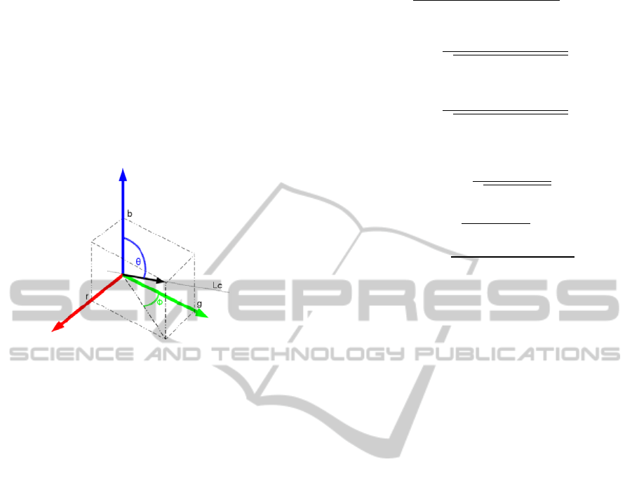
view. In a three-dimensional color space, like RGB,
figure 1 shows the spherical representation of a color
point. A color c with (r,g,b) coordinate values in
RGB color space can be represented by spherical
coordinates
,,
, where and are the angular
parameters and the vector magnitude.
Figure 1: A vectorial representation of color c in the RGB
space.
Spherical coordinates in the three-dimensional RGB
color space can be used to estimate the illumination
source chromaticity, and to detect chromatic edges
(Moreno, Graña, & d'Anjou, 2011; Moreno et al.,
2010). In the three-dimensional RGB color space,
there is a direct correspondence between angular
parameters , and chromaticity (Moreno et al.,
2011).
The angular parameters define a line which is
the natural characterization of the pixel chromaticity.
In other words, all points on this line have the same
chromaticity with the pixel. The spherical expression
of a point in Euclidean space allows to separate
intensity and chromaticity, where l is the intensity,
and the angular parameters provide a
representation/codification of the pixel's
chromaticity.
2.1 Hyperspherical Coordinates
Let us denote p hyperspectral pixel color in n-
dimensional Euclidean space. In Cartesian
coordinates it is represented by
pv
,v
,v
,…,v
where v
is the coordinate value of the i-th
dimension. This pixel can be represented in
Hyperspherical coordinates
,
,
,
,…,
,
where is the vector magnitude that gives the radial
distance, and
,
,
,..
are the angular
parameters. This coordinate transformation is
performed uniquely by the following expression, for
all cases except the ones described below:
⋯
⋯
⋯
⋮
2
Exceptions: if
0for some i but all of
,
,…
are zero then
0. When all
,…,
are zero then
is undefined, usually a
zero value is assigned.
A more compact notation for the hyperspherical
coordinates is ,
where
is the vector of
size n-1 containing the angular parameters. Given a
hyperspectral image
,
,…
;∈
,
where x refers to the pixel coordinates in the
image domain, we denote the corresponding
hyperspherical representation as;
,
;∈
, from which we use
as the chromaticity
representation of the pixel's and
as its (grayscale)
intensity.
To clarify the meaning of the chromaticity in the
hyperspectral image domain, we give an illustrative
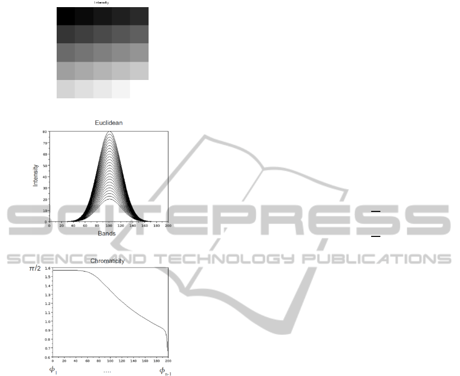
example. We have generated a synthetic
hyperspectral image of 5 x 5 pixels and 200 spectral
bands. Each pixel spectral signature has the same
Gaussian shaped profile but with different peak
height, corresponding to different image intensity as
can be appreciated in Fig. 2(a) showing the image
intensity
. Fig. 2(b) shows the spectral signature of
all pixels in the Cartesian coordinate representation,
Fig.2(c) shows the chromatic spectral signature
which is the same plot for all pixels. The
chromaticity
thus defines a line in the n-
dimensional space of hyperspectral pixel colors of
points that only vary their luminosity .
According to the aforegoing coordinate
transformation, we can perform the following
hyperspectral separation. Given a hyperspectral
image
,
,…
;∈
in the
traditional Cartesian coordinate representation we
can compute the equivalent hyperspherical
representation
,
;∈
. Then, we can
ICPRAM 2012 - International Conference on Pattern Recognition Applications and Methods
434
(a)
(b)
(c)
Figure 2: Synthetic image (a) the image intensity
, (b)
shows the Gaussian shaped signature profile of all the
pixels, and (c) shows the angle components of the
Hyperspherical coodinates shared by the spectral
signatures of all pixels in the image, corresponding to the
common chromaticity of the pixels.
construct the separate intensity image
in Fig
(a). This separation allows us the independent
processing of hyperspectral color and intensity
information, so that segmentation algorithms
showing color constancy can be defined in the
hypespectral domain. This decomposition can be
also embedded in models of reflectance like the
Dichromatic Reflection Model (Shafer, 1984) of the
Bidirectional Reflection Distribution Function where
they can be decomposed as diffuse and specular
components.
3 GRADIENT OPERATORS
Mathematically, the gradient of elements of a
bidimensional space domain function (like images)
is given at each image domain point by the function
derivative given by its horizontal and vertical
Cartesian coordinates, which are the partial
derivatives in these directions. Partial derivatives are
often computed by linear convolution operators. The
gradient function measures the rate of change of the
function in a point. Gradients are easily computed on
the intensity image, but their extension to high
dimensional images is an open research issue.
Let us denote xi,j the pixel coordinates in
the image domain. We recall the definition of the
image spatial gradient:
,
,
,
,
,
where I(i,j) is the image intensity function at
pixel (i,j). For edge detection, the usual convention
is to examine the gradient magnitude:
,
|
,
|
,
For color images, a simplistic approach to
perform edge detection is to drop all color
information, and convolve the intensity image with a
pair of high-pass convolution kernels to obtain the
gradient components and gradient magnitude. The
simplest edge detectors are the Prewitt detectors, is
illustrated in Fig.3 because we will build our own
spatial chromatic gradient operators following their
pattern. To take into account spectral information,
the straightforward approach is to apply the gradient
operators to each spectral band as an independent
intensity image and to combine the results
afterwards I
∑
I
/n
where I
denotes the i-th
image spectral band.
1 0 1
1 0 1
1 0 1
1 1 1
000
111
Figure 3: Prewitt mask.
Fig. 4 shows the results of this approach using
Prewitt gradient operators on two hyperspectral
images (The first one is a plastic blue ball in front of
a green background, the second one is a plastic
orange ball in front of the same green background.
Both images captured under natural sun
illumination). The first row shows one band of the
images. Second row shows the gradient magnitude.
ABOUT GRADIENT OPERATORS ON HYPERSPECTRAL IMAGES
435
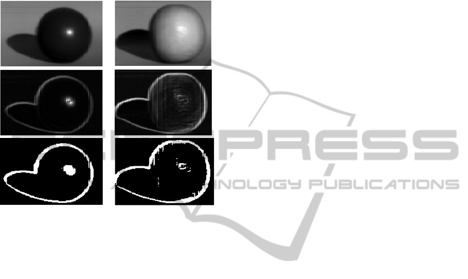
The third row shows some edges detected applying a
threshold to the gradient magnitude image. The
intensity image component has a strong influence on
this gradient computation, therefore some highlights
and shadows are identified as image regions and
their boundaries detected as image edges.
Figure 4: Results on two hyperspectral images of image
gradient computed applying the Prewitt gradient operators
to each band independently.
3.1 Chromatic Gradient Operator
Linear convolution gradient operators, such as the
Prewitt operators shown in Fig. 4, the underlying
topology is the one induced by the Euclidean
distance defined on the Cartesian coordinate
representation. In order to define a chromatic
gradient operator, we may assume a kind of non-
linear convolution where the convolution mask has
the same structure as the Prewitt operators, but the
underlying chromatic distance is based only on the
chromaticity as follows: For two pixels and we
compute the Manhattan or Taxicab distance on the
chromatic representation of the pixels:
∠
p,q
ϕ
,
ϕ
,
Note that the ∠
,
distance is always
positive. Note also that the process is non linear, so
we can not express it by linear convolution kernels.
The row pseudo-convolution operator is defined as
CR
i,j
∠
,
,
,
and the column pseudo-convolution is defined as
CR
i,j
∠
,
,
,
so that the color distance between pixels substitutes
the intensity subtraction of the Prewitt linear
operator. The hyperspectral chromatic gradient
magnitude image is computed as:
(1)
4 EXPERIMENTAL RESULTS
Experiments are performed on images taken by SOC
710 hyperspectral camera. Spectral resolution is 128
bands in the range 300mn to 1000nm. These images
have been presented in the first row of Fig. 4. On
these images we can analyze the illumination effects
over the objects. On these images there are only two
chromatically different surfaces, a uniform green
background and a monochromatic object, in one
case a dark blue ball with a sweet surface; in the
other one is plastic model of an orange. In the
second case, the object has a wrinkled surface.
We have applied the chromatic gradient of eq. 1
on the images. The results are shown in Fig. 5 First
row shows the original intensity images. The second
row shows the chromatic gradient magnitude image.
As we can appreciate, true surface edges are better
detected than in Fig.4 even on shadowy regions of
the image. The highlights have lower response than
in Fig.4, so that no spurious edges are detected
around them. The chromatic gradient has a high
response on the shadows, but this response is
uniformly distributed on the whole shadow and it is
not bigger than the true borders. This effect is
consequence of the noise distribution on the image.
The chromatic distance is more sensitive on region
with poor illumination or on regions poor reflectance
like the blue ball. Comparing these results with the
traditional gradients like the shown on Fig.4, the
chromatic gradient is focused on the chomaticity and
has a bigger response on chromatic edges. Finally,
last row shows the edge detection after applying a
threshold on the gradient magnitude image. The
threshold is computed by the Otsu minimal variance
approach. In these results, we have found the correct
object edges avoiding the false detection of borders
of shines and shadows despite the high dimensional
nature of these hyperspectral images.
ICPRAM 2012 - International Conference on Pattern Recognition Applications and Methods
436
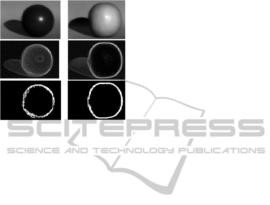
Figure 5: Pseudo Prewitt gradient on the chromatic image.
5 CONCLUSIONS
The computation of gradients on hypespectral
images implies the combination of high dimensional
information and is prone to spurious detections due
to noise and illumination effects, such as highlights
and shadows. We have followed the approach
proposed in (Moreno et al., 2010) for color images,
proposing an extension to high-dimensional images,
which allows the robust detection of object
boundaries despite strong illumination effects. We
have tested the approach on indoors captured
hyperspectral images. Object boundaries are
effectively found and spurious edges are avoided in
these images. Further work on the extensive
validation of the approach on hyperspectral images
with known ground truth is on the way. Long term
research goal is its application to remote sensing
images.
REFERENCES
Cheng, H., Jiang, X., Sun, Y., & Wang, J. (2001, Dec).
Color image segmentation: advances and prospects.
Pattern Recognition, 34(12), 2259–2281.
Gonzalez, R. C., & Woods, R. E. (1992). Digital image
processing (3rd ed.). Addison-Wesley Pub (Sd).
Hildreth, E. C. (1987). Computations underlying the
measurement of visual motion. In (pp. 99–146).
Norwood, NJ, USA: Ablex Publishing Corp.
Moreno, R., Graña, M., & d’Anjou, A. (2011).
Illumination source chromaticity estimation based on
spherical coordinates in rgb. Electronics Letters,
47(1), 28-30.
Moreno, R., Graña, M., & Zulueta, E. (2010, Jun). RGB
colour gradient following colour constancy
preservation. Electronics Letters, 46(13), 908–910.
Shafer, S. A. (1984, april). Using color to separate
reflection components. Color Research and
Aplications, 10, 43-51.
Wang, D. (1997, Dec). A multiscale gradient algorithm for
image segmentation using watershelds. Pattern
Recognition, 30(12), 2043–2052.
ABOUT GRADIENT OPERATORS ON HYPERSPECTRAL IMAGES
437
