VISUALISING SMALL WORLD GRAPHS

Agglomerative Clustering of Small World Graphs around Nodes of Interest

Fintan McGee and John Dingliana

School of Computer Science and Statistics, Trinity College Dublin, Dublin, Ireland

Keywords:

Graph Visualisation, Graph Theory, Clustering Algorithms, Graph Display.

Abstract:

Many graphs which model real-world systems are characterised by a high edge density and the small world

properties of a low diameter and a high clustering coefﬁcient. In the ”small world” class of graphs, the

connectivity of nodes follows a power-law distribution with some nodes of high degree acting as hubs. While

current layout algorithms are capable of displaying two dimensional node-link visualisations of large data sets,

the results for dense small world graphs can be aesthetically unpleasant and difﬁcult to read, due to the high

level of clutter caused by graph edges. We propose an agglomerative clustering which allows the user to select

nodes of interest to form the basis of clusters, using a heuristic to determine which cluster each node belongs

to. We have tested three heuristics, based on existing graph metrics, on small world graphs of varying size and

density. Our results indicate that maximising the average cluster clustering coefﬁcient produces clusters that

score well on modularity while consisting of a set of strongly related nodes. We also provide a comparison

between our clustering coefﬁcient heuristic agglomerative approach and Newman and Girvan’s top-down Edge

Betweenness Centrality clustering algorithm.

1 INTRODUCTION

Many real-world networks across different ﬁelds have

similar characteristics and can be classiﬁed as small

world graphs (Watts and Strogatz, 1998). Small world

networks are characterised by two properties. The

ﬁrst is the average of the shortest path between each

pair of vertices for the entire graph. The second prop-

erty is the average local clustering coefﬁcient of the

graph, which is deﬁned as the average of the clus-

tering coefﬁcients for each vertex. Given an undi-

rected graph G = (V,E), where V is a set of vertices

...v

} and E is a set of edges e ∈ E connect-

ing vertices x ∈ V and y ∈ V with e(x,y) = e(y, x), the

neighbourhood of a vertex v, denoted Γ

is deﬁned

as the set of all vertices adjacent to v, not including

v itself. The clustering coefﬁcient for a vertex , de-

noted by γ

is most commonly deﬁned as the ratio

of edges connecting the neighbours of a vertex to the

maximum number of edges that could possibly con-

nect the neighbours of the vertex (Watts, 2003). The

clustering coefﬁcient c for a vertex v in an undirected

graph is given by

|E(Γ





(1)

where |E(Γ

)| is the magnitude of the set of edges

connecting neighbours of the vertex, k is the neigh-

bourhood size of the vertex, i.e.|Γ

|and





is the

maximum possible number of edges in Γ

. From

the above it can be seen that a vertex needs at least

two neighbours to have a valid clustering coefﬁcient

value. To determine if a graph can be considered a

small world graph, it is compared to a randomly gen-

erated graph with the same number of vertices and

edges. A small world graph has approximately the

same average path length, but a considerably higher

(by orders of magnitude) clustering coefﬁcient.

1.1 Motivation

Our motivation is to make graphs more comprehen-

sible. We are focusing on small world graphs specif-

ically due to the presence of groups of highly con-

nected nodes and the strong likelihood of clusters

within the graph as well as the common occurrence

of small world properties in real world networks. If

a user has nodes of speciﬁc interest to them, reorgan-

ising the layout of the graph based on the nodes of

interest may aid in their analysis. For example a user

may want to view a graph describing a large program

focusing on speciﬁc classes. The purpose of our clus-

678

McGee F. and Dingliana J..

VISUALISING SMALL WORLD GRAPHS - Agglomerative Clustering of Small World Graphs around Nodes of Interest.

DOI: 10.5220/0003864306780689

In Proceedings of the International Conference on Computer Graphics Theory and Applications (IVAPP-2012), pages 678-689

ISBN: 978-989-8565-02-0

 2012 SCITEPRESS (Science and Technology Publications, Lda.)

Figure 1: A small world graph based on the connection be-

tween a small set of Wikipedia articles (|V | = 91|E| = 418)

laid out using a simple force directed algorithm.

tering approach is to aid in the layout by clustering

nodes around the user’s nodes of interest. The cluster-

ing assigns nodes in such a way that they are clustered

around nodes that they are more conceptually related

to. If grouping a node with one node set over another

results in a higher heuristic score for that clusters, we

can infer that the node conceptually belongs more to

that set. In less dense graphs a clustering may be obvi-

ous as there will be few links between clusters. How-

ever for more dense graphs useful clusterings may not

be so obvious and the density of edges can make the

graph more difﬁcult to read. The purpose of this pa-

per is to determine what heuristic is best suited for our

approach to clustering.

1.1.1 Edge Density

The links in a node link visualisation convey impor-

tant information. However if they become too dense

the graph becomes less comprehensible, resulting in

nodes and other links becoming obscured. In terms of

graph theory the density of a graph is usually consid-

ered the ratio of edges to the maximum possible num-

ber of edges in the graph (Coleman and Mor, 1983).

For an undirected graph this can be described as

d =

|E|

|(V |(|V | − 1)/2)

(2)

A graph is then considered dense in theoretical terms

if this ratio approaches 1.0. However in practical

real world examples of information visualisation such

dense graphs are rarely seen. If we consider the

density of a graph to be the ratio of edges to nodes

= |E|/|V |, often referred to as the linear density,

most real graphs have a value of d

<= 10 (Melan-

con, 2006), however this is still enough to cause a

large amount of clutter. Melacon et al. give an exam-

ple of real world graphs which have even higher den-

sities, such as webcrawl graphs with d

= 25.57. The

Figure 2: The graph from ﬁgure 1 clustered using our ap-

proach around the four most well connected nodes, us-

ing clustering coefﬁcient as a clustering heuristic, and

bundling(Holten, 2006) of inter-cluster edges.

graph in ﬁgure 1 has a density value d

= 4.59, which,

while not the most dense example, still appears difﬁ-

cult to read due to the number of edges. It is clear that

graph theoretic density scales the number of edges

more dramatically for a change in vertex count, so for

comparison of densities between graphs with different

node counts linear density provides a clearer result.

However for understanding the impact of density on

graphs with a constant node count, the graph theoretic

density is clearer as it does scale evenly between the

maximum and minimum edge count. Purchase (Pur-

chase, 1997) has demonstrated how the crossing of

edges is the graph aesthetic which affects most hu-

man understanding of the graph. Unfortunately in

large dense graphs edge crossings are unavoidable.

We hope that by clustering the graph intelligently,

strongly related nodes will appear closer to each other

within the same cluster. This will reduce long edges

and the likelihood of edge crossings.

2 RELATED WORK

2.1 Small World Graphs

Milgram (Milgram, 1967) ﬁrst described small world

graphs in his work focused on social networks. The

concept was more recently revived by (Watts and

Strogatz, 1998) and has been shown to hold true for a

variety of networks, such as the relationships between

actors and ﬁlms (Auber et al., 2003) as well as com-

puter systems (Cai-Feng, 2009), models of biological

networks(Watts and Strogatz, 1998) and citation net-

works (van Ham, 2004).

VISUALISING SMALL WORLD GRAPHS - Agglomerative Clustering of Small World Graphs around Nodes of Interest

679

2.2 Clustering

(Eades and Feng, 1997) describe clustered graphs as

graphs with recursive clustering structure over the

vertices. In their example the clustering structure is

an attribute of the graphs and vertices. However in

many cases, if a graph is to be clustered, there may

be no intrinsic attribute or parameter which describes

the clustering hierarchy. There are many different ap-

proaches to generating an optimum clustering as it

is a difﬁcult problem that is NP-complete (Newman

and Girvan, 2004). Approaches to graph clustering

can be considered geometric or non-geometric. The

aim of geometric clustering is to have vertices that

are geometrically close to each other share a cluster

and vertices that are distant from each other appear

in separate clusters. An example of such a cluster-

ing is given by Quigley and Eades’ FADE algorithm

(Quigley and Eades, 2001) in which a quad-tree is

used alongside a modiﬁed force directed algorithm.

There are many different methods of non-geometric

clustering. Some methods such as Markov Cluster-

ing (MCL) (Van Dongen, 2000) and spectral portion-

ing (Frishman and Tal, 2007) use an algebraic ap-

proach, working on a mathematical representation of

the graph. Other methods such as Edge Betweenness

Centrality Clustering (Newman and Girvan, 2004)

use a graph based approach, calculating properties of

vertices or edges that are then used to partition the

graph into clusters. Quigley and Eades’ geometric

approach can be considered a bottom up (agglomer-

ative) approach while Newman and Girvan’s is con-

sidered top-down (divisive) approach. An agglomera-

tive clustering algorithm merges set of nodes together

to form clusters, a divisive approach divides the full

set of nodes into clusters. Schaeffer (Schaeffer, 2007)

provides an in depth review of clustering methods and

methods for evaluating cluster quality.

2.2.1 Clustering Evaluation

Newman and Girvan (Newman and Girvan, 2004) de-

ﬁne a measure of the quality of a division of a net-

work graph, referred to as modularity. The measure

is used to evaluate their community detection algo-

rithm (which is essentially a top-down clustering al-

gorithm). The measure has also been used in work

by Newman (Newman, 2004) as a heuristic value for

building clusters. This metric is based upon the num-

ber of edges that start and end in the same cluster (re-

ferred to as communities in Newman and Girvan’s pa-

per). Auber et al (Auber et al., 2003) and Chiricota et

al. (Chiricota et al., 2003) use a quality measure de-

veloped by (Mancoridis et al., 1998) and utilised in

their clustering tool ”Bunch”. This measure, denoted

MQ (Modularisation Quantity) computes a value for

any given partition of a graph. Chiricota et al. and

Auber et al. use a slightly modiﬁed version of MQ

that is deﬁned only for undirected graphs as an eval-

uation measure. The MQ value is used by the Bunch

tool as a function to be optimised to provide a good

clustering, rather than as a metric to evaluate one.

Boutin and Hascoet (Boutin and Hascoet, 2004) dis-

cuss many clustering evaluation approaches (referred

to by them as clustering validation indices) and they

note that these evaluations are often difﬁcult to inter-

pret and compare.

Difference between Modularity and Modularisa-

tion Quantity. The MQ metric differs to Newman

and Girvan’s modularity measure. The latter com-

pares the fraction of all edges that are intra-cluster

edges to the fraction of all edges that are inter-cluster

edges. The former is a measure of the difference be-

tween the average ratio of actual intra-cluster edges

to the maximum amount of intra-cluster edges possi-

ble and the average ratio of the amount of inter-cluster

edges to the maximum amount of inter-cluster edges

possible. This means that modularity depends purely

on the number of edges, which is bounded to the num-

ber of nodes. MQ depends on the number of edges

and the number of nodes directly, as the maximum

possible number of edges between two clusters is a

function of the number of vertices.

3 PROPOSED APPROACH

Our approach consists of an agglomerative clustering

algorithm, focused on nodes of interest selected by

the user. We grow the clusters around each of these

nodes of interest by adding nodes based on a heuristic

evaluation of the quality of the resulting clustering of

the graph.

3.1 Chosen Heuristics

Modularity. Per Newman and Girvan (Newman

and Girvan, 2004) the modularity, Q, is calculated as

Q =

∑

i −a

) (3)

Where e

i is the fraction of all edges that start and

end in cluster i and a

is the fraction of all edges that

terminate in cluster i. A modularity score of 1.0 indi-

cates that all edges are intra-cluster edges, a score of

0.0 indicates the clustering is equivalent to a random

one. Newman (Newman, 2004) uses modularity as a

guiding heuristic for a greedy agglomerative cluster-

ing process.

IVAPP 2012 - International Conference on Information Visualization Theory and Applications

680

Modularisation Quantity (MQ). We calculate MQ

using Auber et al’s approach (Auber et al., 2003) for

undirected graphs. Let A and B be two sets of disjoint

nodes in a graph G = (V,E) , let s equal the ratio of

edges between the two sets to the maximum possible

number of edges between the two sets.

s(A,B) =

|E(A,B)|

|A| ·|B|

(4)

Note that this ratio can be calculated for a set with

itself. For a cluster A in an undirected Graph without

self linking edges

s(A,A) =

2(|E(A,A)|)

|A| ·(|A| − 1)

(5)

If cluster A is a clique s(A,A) = 1. A clique is a set of

nodes where every node is connected to every other

node in the set. If none of the nodes in A are con-

nected s(A,A) = 0. If a cluster contains only a sin-

gle node, we deﬁne the s-value for that cluster to be

0. Given a partition ( also referred to as a clustering)

C = (C

,....,C

) that divides the graph G = (V,E)

into p partitions the MQ score for that partition is

given by:

MQ(C;G) =

∑

i=1

s(C

)

−

∑

p−1

i=1

∑

j=i+1

s(C

)

p(p −1)/2

(6)

Essentially this is a measure of the difference be-

tween the s ratio of intra-cluster edges (denoted by

s(C

) and the s ratio of inter-cluster edges (denoted

by s(C

Clustering Coefﬁcient. The clustering coefﬁcient

of a graph is described in section 1. When we cal-

culate the average clustering coefﬁcient of a cluster,

we only consider the nodes and their neighbours from

within that cluster. The average clustering coefﬁcient

of a cluster describes how well inter-connected the

cluster is. This implies that the higher the cluster-

ing coefﬁcient of a cluster the more strongly related

the nodes within the cluster are. Unlike the previous

two metrics, this metric only applies to a single cluster

and not to all of the clusters so far deﬁned within the

graph. Therefore a high average of the average clus-

tering coefﬁcient for each cluster does not imply that

all clusters have a high average clustering coefﬁcient.

A large standard deviation between the average clus-

tering coefﬁcients of the clusters indicates that some

clusters have been created with a low quality of clus-

tering. In the cases where a clustering using a heuris-

tic other than clustering coefﬁcient produces clusters

containing only one or two nodes, it is not possible to

calculate the average clustering coefﬁcient of the clus-

ter so we assign the cluster a clustering coefﬁcient of

-1.0. This results in a suitably decreased score that re-

ﬂects to poor quality of the clustering, when rating the

graph using the average cluster clustering coefﬁcient.

Random Assignment. In order to provide a com-

parison clustering in which no heuristic is used, we

have also implemented a random assignment of nodes

to clusters. A node is chosen at random from the

combined neighbourhood of the clusters and then ran-

domly assigned to one of the clusters that it is con-

nected to. The process is then repeated until all nodes

are assigned. Nodes can only be assigned to clusters

in which they have a neighbour, to allow a reasonable

comparison with the preceding heuristics.

3.2 Initial Cluster Set Up

The initial set of nodes that are to form the basis of

the clustering is selected by the user. We term these

nodes supernodes. If our heuristic is either modularity

or MQ, or we are using the random approach, we can

begin to add further nodes to the clusters once the ini-

tial cluster nodes have been speciﬁed. This is because

it is possible to calculate modularity and MQ heuris-

tic value, or randomly choose a node, if a cluster con-

tains only 1 node. However this is not the case for the

clustering coefﬁcient heuristic, as we need to have at

least two nodes existing already in the cluster before

we can calculate a valid heuristic value for a new node

being added. Therefore, before we start adding candi-

date nodes to the cluster using clustering coefﬁcient as

a heuristic we need to add a second node to the cluster

of each of the supernodes. The nodes that are consid-

ered to be added are nodes within the neighbourhood

of the supernode. We would like to add a node that is

similar as possible to each of the supernodes, so we

use the Jaccard index of the supernode and the can-

didate second node’s respective neighbourhoods. The

Jaccard index of two sets of nodes A and B, ρ is de-

ﬁned as:

ρ(A,B) =

|A| ∩|B|

|A| ∪|B|

(7)

If the super-node is denoted by v and the candidate

node is denoted by u we can write the Jaccard index

ρ(Γ(v),Γ(u)) =

Γ(v) ∩Γ(u)

Γ(v) ∪Γ(u)

(8)

The node which is used as the secondary node of

the cluster based around v is the node u for which

ρ(Γ(v),Γ(u)) is the largest. Ideally we aim to se-

lect a node where the neighbourhood Jaccard index

is 1. If the node chosen has already been assigned as

a neighbour of one of the other supernodes, we as-

sign the node to the supernode which results in the

VISUALISING SMALL WORLD GRAPHS - Agglomerative Clustering of Small World Graphs around Nodes of Interest

681

Figure 3: An example considering whether the green node

should be clustered with either the red or blue clusters us-

ing the clustering coefﬁcient heuristic. The green node is

added to the blue cluster increasing the cluster’s local av-

erage clustering coefﬁcient to 0.48. Adding it to the red

cluster would reduce its average local clustering coefﬁcient

to 0.33.

best Jaccard neighbourhood index. The supernode

with the lower resulting Jaccard index is assigned the

node with the next highest resulting Jaccard index. If

this replacement node has also been assigned, we re-

peat the revaluation until all supernodes have been as-

signed distinct neighbours.

3.3 Assignment of Nodes to Clusters

Once the initial clusters are created, we store the

neighbourhood of each cluster and use this as input set

of nodes which can be potentially added to a cluster.

Given a clustering of p clusters C = (C

,....,C

)

where each element of C contains a disjoint subset

of the graph G = (V,E) such that C

= v

,...v

n = |C

| and C

⊂ V , we deﬁne the neighbourhood of

a cluster i as

Γ(C

) = (Γ

) ∪Γ

)... ∪Γ

)) (9)

Each of the candidate nodes is added temporarily to

a cluster and a score based on that addition is calcu-

lated. The node which maximises the heuristic score

of the graph (or of each cluster) is permanently added

to the cluster. Once a node is added the process is

repeated until all nodes have been assigned to clus-

ters. The modularity and MQ heuristics are scored

for the graph as a whole, so once a node is added all

scores will have to be recalculated in the next round

of assignments. If the clustering coefﬁcient heuristic

is being used, only the cluster average clustering coef-

ﬁcient of the cluster which has had a node added will

have changed. The average clustering coefﬁcients

calculated for the other clusters and their candidate

nodes will be unchanged from previous rounds. This

allows caching of the results for later reuse, therefore

it decreases computation time.

4 EVALUATION

4.1 Evaluation Graphs

We use Watts and Strogatz’s beta approach for cre-

ating small world graphs (Watts and Strogatz, 1998)

for evaluating the effectiveness of the heuristics. This

approach allows us to create a large set of graphs

of various densities and various levels of structure,

from regular lattices, to small worlds graphs, to com-

pletely random graphs. The approach begins by cre-

ating a lattice like structure with edges uniformly dis-

tributed across vertices, k edges per-vertex resulting

in |E| = k|V |. Each edge is rewired to a random target

vertex with a probability P. For a low value of P the

resulting graph is well structured and exhibits small

world properties. As P approaches 1 the graph be-

comes more like a randomly connected graph. Each

graph in our test set consists of 200 vertices. We have

generated graphs varying the input probability to the

beta model from 0.5 to 0.95. We have also varied

the Edge density of the graph from a graph theoretic

value of value of d = 0.015 to d = 0.3 , resulting in the

most dense graph having 11,940 edges. This is equiv-

alent to a range of linear edge densities from d

= 1.49

to d

= 29.85. We have clustered each graph using

our described heuristics. For evaluating the graphs

we also rate them using the MQ score and modular-

ity score of the resulting clustered graph, as well as

examining the average of per cluster average cluster-

ing coefﬁcients and the standard deviation of the per

cluster average clustering coefﬁcient. The four nodes

with the largest neighbourhoods have been selected as

the nodes of interest, resulting in four clusters. Due to

the random nature of the graph generation we have

averaged each result across 3 graphs generated with

the same input parameters. Our full test set of data

consist of 285 graphs for each of the three generation

runs. We display the results of the clustering for a

sample of the low density graphs in ﬁgure 4, a sample

of the high density graphs in ﬁgure 5, a sample of the

more structured graphs in ﬁgure 6 and a sample of the

more random graphs in ﬁgure 7. The standard devia-

tion of the heuristics across the 3 graphs is displayed

as the error bounds.

4.2 Results and Analysis

The effectiveness of each heuristic differs depending

on the density of the graph, how random the graph

is as a result of the input probability p of the gener-

ation algorithm, and the metric used for evaluation.

There are some constants however. Throughout the

graphs displayed in ﬁgures 4 through 7 it can be seen

IVAPP 2012 - International Conference on Information Visualization Theory and Applications

682

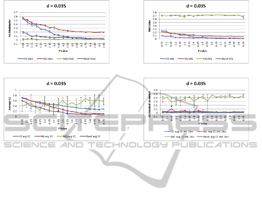
(a) Resulting graph modularity for each heuristic. (b) Resulting graph MQ score for each heuristic.

for each heuristic.

(d) The standard deviation of the average cluster

clustering coefﬁcient of each of the four clusters

for each heuristic.

Figure 4: Evaluation of graphs with 200 Nodes and a density of 0.035 (d

= 3.483), and an increasing level of randomness,

denoted by p value.

that the random approach of assignment of nodes to

clusters generally scores close to zero when evaluated

using modularity or MQ. This is to be expected as

both of these metrics lie in the range [−1,1] with zero

being equivalent to a random clustering. In the less

dense graphs sometimes the random approach does

score slightly above zero for a low input probability p,

when the graphs are less random. This is because of

the fact that our random approach does rely on nodes

to be connected to the clusters they are added to, re-

ducing the number of options for less well connected

nodes. For higher density graphs this is not evident

as a node will have a larger set of clusters it can be

assigned to. It is clear from each of these ﬁgures that

a graph scores well when it is rated with a metric that

is also used as the heuristic to build the clusters. It

also seems surprising that using MQ as a heuristic

results in a high average per cluster clustering coef-

ﬁcient, however looking at the standard deviation of

the per cluster clustering coefﬁcients shows that the

individual clusters vary wildly in quality. This is a re-

sult of a very imbalanced clustering, which will not be

of beneﬁt to a user if the majority of nodes are placed

in a cluster with a low average clustering coefﬁcient.

This means that the nodes within the cluster will be

less strongly related to each other.

4.2.1 Low Density Graphs

Figure 4 shows the resulting modularity, MQ and

clustering coefﬁcient values when the algorithm is run

on graphs of increasing randomness with a relatively

low density, d = 0.035,d

= 3.483. Due to the rela-

tively low density, there are fewer nodes to be chosen

from when adding new nodes to the clusters, so nodes

being added to a cluster are more likely to closely re-

late to several of the other nodes within the cluster.

This is reﬂected by the higher scores for the random

layout approach for each heuristic for a low levels of

rewiring probability, see ﬁgure 4. Rating the graph

based on modularity (ﬁgure 4a) results in the best

results for the modularity heuristic with the cluster-

ing coefﬁcient approach not far behind. The MQ ap-

proach noticeably scores similarly to the random ap-

proach. Rating the graph based on MQ (ﬁgure 4b)

results in a consistently high score regardless of the

level of randomness when using MQ as a heuristic.

Using the average cluster clustering coefﬁcient as a

heuristic results in a low score of 0.2 for the more

structured graphs, but this diminishes toward 0.0 as

the graph becomes more random, making it no more

effective than the random approach. The modularity

heuristic scores similarly to the clustering coefﬁcient

VISUALISING SMALL WORLD GRAPHS - Agglomerative Clustering of Small World Graphs around Nodes of Interest

683

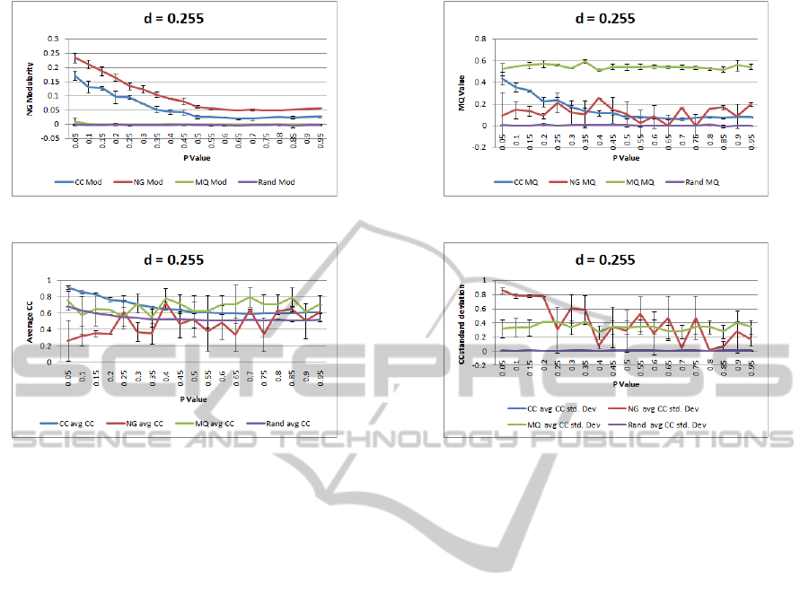
(a) Resulting graph modularity for each heuristic. (b) Resulting graph MQ score for each heuristic.

cient for each heuristic.

(d) The standard deviation of the average cluster

clustering coefﬁcient of each of the four clusters

for each heuristic.

Figure 5: Evaluation of a graphs with 200 Nodes and a density of 0.255 (d

= 25.3725), and an increasing level of randomness,

denoted by p value.

heuristic, for structured graphs and also diminishes,

but to a lesser degree than the clustering coefﬁcient

approach. Rating the graph using average cluster

clustering coefﬁcient (ﬁgure 4c), we can see that clus-

tering coefﬁcient and modularity perform similarly

for structured graphs and diverge as the graphs be-

come more random. We can also see from the error

bounds that the MQ heuristic produces varying re-

sults for each of the 3 input graphs, where the other

approaches are consistent in their results. Even with

the large error bounds, once the graph becomes suf-

ﬁciently random, MQ appears to provide the highest

average clustering coefﬁcient of the resulting clusters,

but if we look at the standard deviation of the average

clustering coefﬁcient of each of the clusters created

by the MQ heuristic (ﬁgure 4d), we can see that the

quality of the clustering is quite poor. A large stan-

dard deviation of the average of the clustering coefﬁ-

cients of the 4 clusters indicates that while some clus-

ters have a high clustering coefﬁcient others will have

a very poor one. This means the MQ does not in fact

provide a good consistent average cluster clustering

coefﬁcient, therefore clusters will be created where

adjacent nodes do not have many mutual neighbours,

and will be less conceptually alike.

Conclusions: For graphs of low density clustering

coefﬁcient and modularity are the preferred heuristics

when the graph contains structure. As the graphs be-

come more random modularity becomes the sole pre-

ferred heuristic.

4.2.2 High Density Graphs

Changing the density of the graph has an impact on

the performance of each of the heuristics. Figure

5 show results for graphs with a high density, d =

0.255,d

= 25.3725199. Rating the graphs based on

modularity (ﬁgure 5a), we see that overall the scores

are lower when compared to the less dense graphs,

however the same trends hold true as for the lower

density graphs. Rating the graphs based on MQ score

(ﬁgure 5b), we again see the MQ heuristic perform

well. A noticeable difference is the improved perfor-

mance of the clustering coefﬁcient heuristic for the

more structured graphs. The modularity metric per-

forms better relative to clustering coefﬁcient as graphs

become more random, but the scores are less con-

sistent, with larger standard deviations. Rating the

graphs based on average cluster clustering coefﬁcient

results in the clustering coefﬁcient heuristic perform-

ing the best for the more structure graphs. As the

graphs become more random, the MQ heuristic per-

IVAPP 2012 - International Conference on Information Visualization Theory and Applications

684

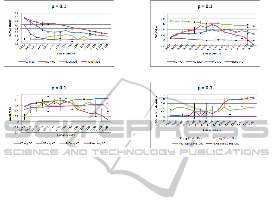
(a) Resulting graph modularity for each heuristic. (b) Resulting graph MQ score for each heuristic.

for each heuristic.

(d) The standard deviation of the average cluster

clustering coefﬁcient of each of the four clusters

for each heuristic.

Figure 6: Evaluation of a graph with 200 Nodes and a constant input rewiring probability p = 0.1, and an increasing density.

formance does appear to perform slightly better, but

the larger standard deviation in results across the in-

put graphs reveals it does not do so. Also, as for the

less dense graphs, the standard deviation of the av-

erage clustering coefﬁcient (ﬁgure 5d) of each clus-

ter is much higher than the clustering coefﬁcient ap-

proach. It is noticeable that for most of the graphs the

modularity heuristic performs even worse than using

the random approach and that the clusters generated

vary largely in average clustering coefﬁcient. Conclu-

sions: Clustering Coefﬁcient is the most consistently

high performing heuristic across all metrics. Modu-

larity results in a large deviation in the average clus-

tering coefﬁcient of individual clusters within a graph

as long as there is some structure in it. As the graph

approaches random, modularity performs similarly to

clustering coefﬁcient, but there is not enough differ-

ence to recommend it above clustering coefﬁcient.

4.2.3 Low Randomness Graphs

These are the graphs which exhibit small world prop-

erties. Rating the graphs based on modularity (ﬁg-

ure 6a), we see the modularity heuristic score best as

expected, however the score decreases as the graphs

become more dense. The average clustering coefﬁ-

cient scores best out of the other heuristics and also

decreases similarly to the modularity approach as the

graphs become more dense. Using MQ as a heuris-

tic, modularity behaves erratically, with large error

bars and scores worse than random for the less dense

graphs, and similar to random for the more dense

graphs, with a large standard deviation. Rating the

graphs based on MQ (ﬁgure 6b), we see the expected

high score for MQ. Interestingly we see low scores

for modularity for both the less dense and most dense

graphs, however for graphs in the mid range of densi-

ties it does improve considerably, just about outper-

forming the clustering coefﬁcient approach. Look-

ing at the average cluster clustering coefﬁcient (ﬁgure

6c), we see clustering coefﬁcient performs the best

at all densities, with close competition from modu-

larity at lower graph densities. The average cluster

clustering coefﬁcient rating for the MQ heuristic still

exhibits a large standard deviation between individual

clusters (6b) for all densities. For more dense graphs,

the use of modularity as a heuristic performs quite

poorly.

Conclusions: The clustering coefﬁcient heuristic

performs relatively well across all levels of density

for all metrics. The closest rival is modularity, which

is similarly effective until a density of approximately

0.19 (d

= 18.905) is reached.

VISUALISING SMALL WORLD GRAPHS - Agglomerative Clustering of Small World Graphs around Nodes of Interest

685

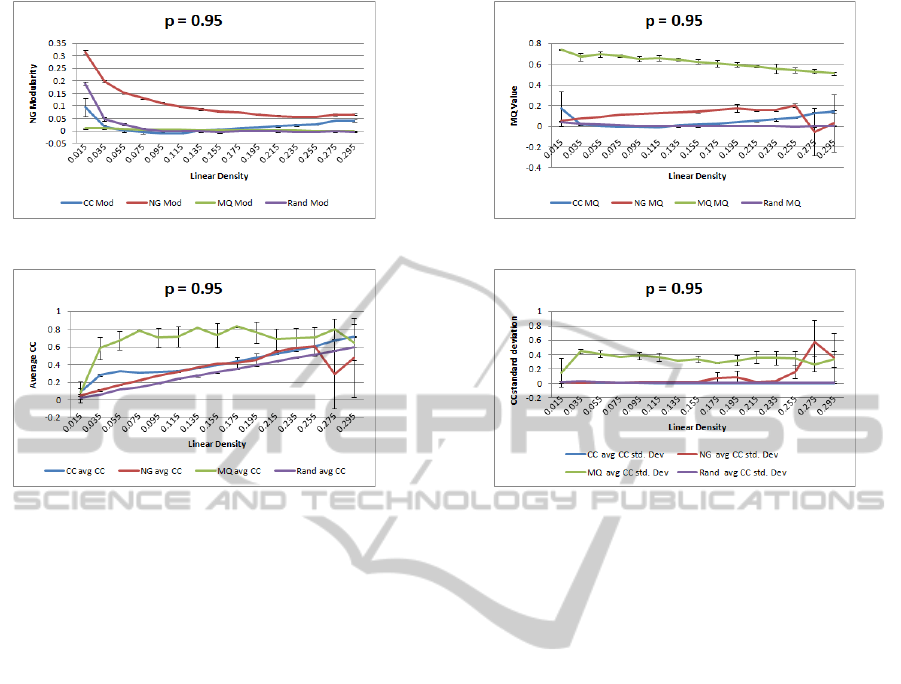
(a) Resulting graph modularity for each heuristic. (b) Resulting graph MQ score for each heuristic.

for each heuristic.

(d) The standard deviation of the average cluster

clustering coefﬁcient of each of the four clusters

for each heuristic.

Figure 7: Evaluation of a graph with 200 Nodes and a constant input rewiring probability p = 0.95, and an increasing density.

4.2.4 High Randomness Graphs

These are the graphs which exhibit a high level of ran-

domness, and thus exhibit no small world properties.

These graphs can give us insight into what approaches

are affected most by the absence of a high cluster-

ing coefﬁcient. All heuristics other than modularity

perform poorly when rated using graph modularity

(ﬁgure 7a). Rating the graph using MQ (ﬁgure 7b),

we see, as expected, MQ performs very well, with

modularity performing poorly but better than random

or the clustering coefﬁcient heuristic. When we rate

the graphs using average cluster clustering coefﬁcient

(ﬁgure 9c) we see that there are some small improve-

ments over random using modularity and clustering

coefﬁcients as heuristics, and that as graph density in-

creases the scores for these approaches increases in a

manner similar to the random approach. This is to be

expected given the random nature of the graph. From

this ﬁgure and ﬁgure 5b, we can see that when using

MQ as a heuristic and rating the ﬁnal clustered graph

using MQ, the results are not reliable as they appear to

be independent of graph randomness and only slightly

affected by graph density.

Conclusions: Overall the best heuristic for graphs

which are more random and less structured appears

to be modularity, until the graphs become very dense

d = 0.26,(d

= 25.87), when average clustering coef-

ﬁcient becomes marginally better.

4.2.5 Comparison with Edge Betweenness

Centrality Clustering

To provide a comparison with a state of the art cluster-

ing approach we performed a similar analysis on our

test data set having applied Edge Betweenness Cen-

trality clustering (Newman and Girvan, 2004). This

is a top town clustering approach which tries to ﬁnd

naturally occurring clusters within the data. Unlike

our approach, the number of clusters is not usually

speciﬁed and there is no equivalent of a user specify-

ing nodes of interest. However it is an effective algo-

rithm which can distinguish the clusters which natu-

rally occur within a small world graph. The algorithm

generates a hierarchy of partitions. The partitioning

with the best modularity score is chosen from this hi-

erarchy as the ﬁnal clustering. This can result in a

high number of clusters depending on the density and

structure of the graph, as can be seen in ﬁgure 10. In

many cases a very large number of clusters are cre-

ated, thus for our comparison we are constraining the

number of clusters formed by the Newman and Gir-

van approach to 4, the same number used for our ag-

glomerative clustering analysis. Evaluation uses the

same approach as that used for evaluating our cluster-

ing heuristics and the results can be seen in ﬁgures 8

IVAPP 2012 - International Conference on Information Visualization Theory and Applications

686

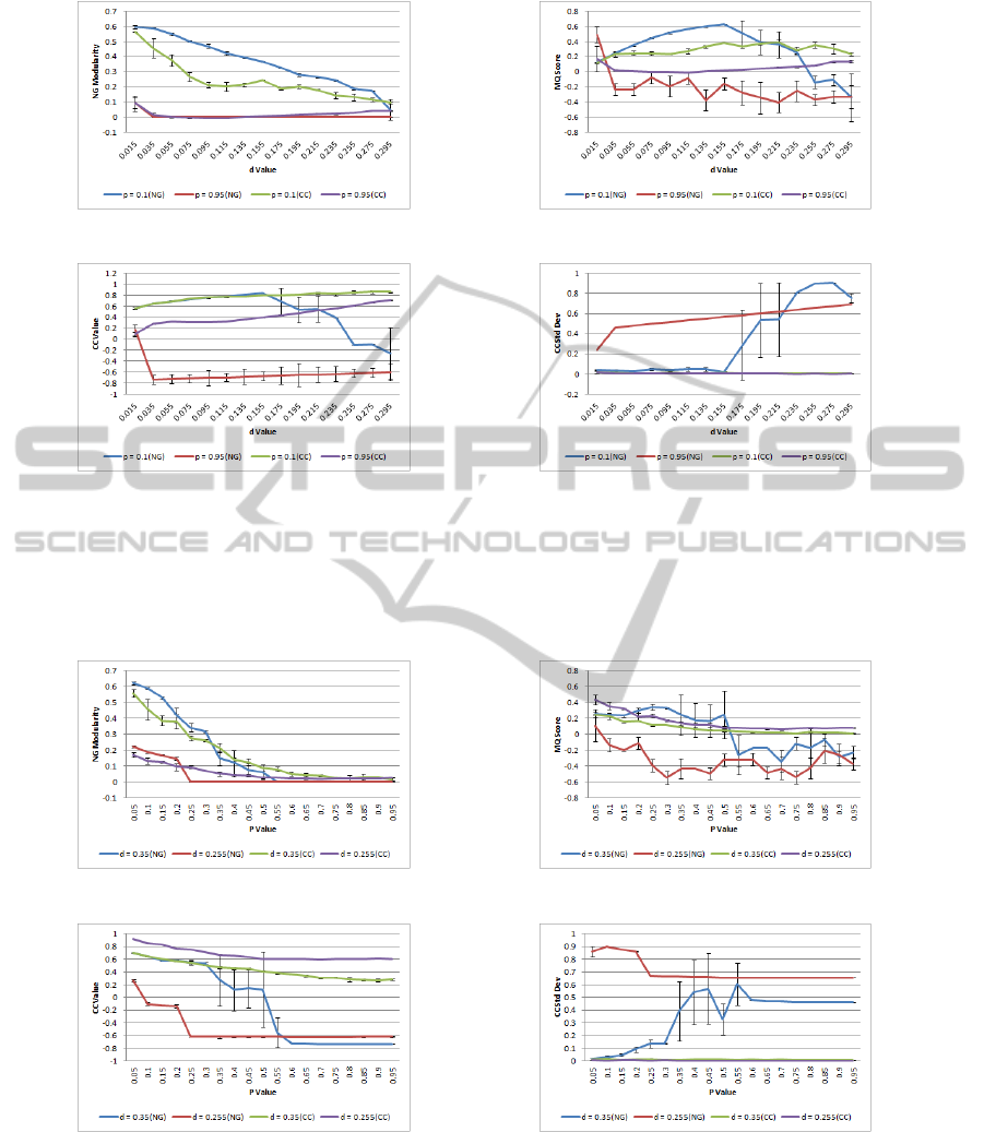
(a) Graph Modularity. (b) Graph MQ score.

of the 4 clusters.

(d) The standard deviation of the average

cluster Clustering Coefﬁcient of each of

the clusters.

Figure 8: Evaluation of test graphs when clustered using Newman and Girvan’s Edge Betweenness Centrality clustering (NG)

and our clustering coefﬁcient heuristic (CC) for comparison. The graphs display the metrics for well structured (p = 0.1) and

unstructured graphs (p = 0.95) of increasing density, where the number of clusters is constrained to 4.

(a) Graph Modularity. (b) Graph MQ score.

of the 4 clusters.

(d) The standard deviation of the aver-

age cluster clustering coefﬁcient of each

of the clusters for high and low density

graphs, both with and without a predeter-

mined number of clusters.

Figure 9: Evaluation of test graphs when clustered using Newman and Girvan’s Edge Betweenness Centrality Clustering

(NG) and our clustering coefﬁcient heuristic (CC) for comparison. The graphs display the metrics for low density (d = 0.035)

and high density graphs (d = 0.255) with an decreasing level of structure (p increasing), where the number of clusters is

constrained to 4.

VISUALISING SMALL WORLD GRAPHS - Agglomerative Clustering of Small World Graphs around Nodes of Interest

687

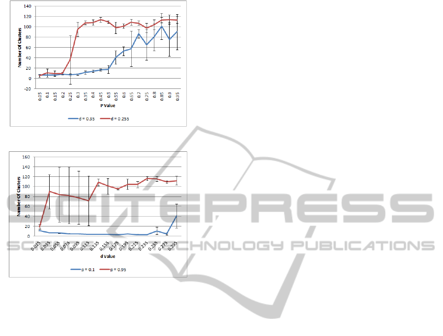
(a) Graphs with a constant density.

(b) Graphs with a constant rewiring probability.

Figure 10: Number of clusters generated using Edge be-

tweenness Centrality Clustering.

and 9.

Less Dense Graphs. When clustering lower density

graphs, compared to cluster coefﬁcient heuristic ag-

glomerative approach, the cluster count limited ver-

sion of Edge Betweenness Centrality lustering pre-

dictably scores higher on modularity (ﬁgure 9a). This

is as the clustering is not constrained by the user spec-

ifying supernodes to form the basis of clusters and

the algorithm is very effective at ﬁnding the small

amount of clusters in the more structured graphs (see

ﬁgure 10). Predictably as the graph becomes more

random this difference diminishes until the cluster co-

efﬁcient approach produces cluster with a higher level

of modularity, as there are fewer naturally occurring

communities for more random graphs. For the MQ

score, (see ﬁgures 9b , 8b) Edge Betweenness Cen-

trality clustering is superior, however the difference is

not as large, and once the graphs become less struc-

tured the performance of the approach drops off sig-

niﬁcantly. In terms of clustering coefﬁcient Edge Be-

tweenness Centrality clustering performs similarly for

the more structured graphs but drops off signiﬁcantly

as the graphs become more random.

More Dense Graphs. From ﬁgure 8 it can be seen

that graphs with stronger small world graph character-

istics modularity is slightly better, but the clustering

coefﬁcient approach performs better once the graphs

become slightly more random (at approximately p =

0.2, so the underlying structure is still quite strong).

However for the MQ score we ﬁnd that, for the more

dense graphs, the clustering coefﬁcient consistently

outperforms the Edge Betweenness Centrality clus-

tering approach. Our approach also provides equiva-

lent and better average clustering coefﬁcient for clus-

ters and far higher clustering coefﬁcient values for

the more random graphs (due to all of the singleton

clusters). Our approach also maintains more consis-

tently high clustering coefﬁcient values for the more

dense graphs (d > 0.235, d

> 23.38) than Newman

and Girvan’s approach. The low standard deviation

between the clustering coefﬁcients also indicates that

the resulting average clustering coefﬁcient is balanced

across multiple clusters.

5 CONCLUSIONS AND FUTURE

WORK

Based on the preceding analysis the most consis-

tently effective heuristic for agglomerative clustering

around nodes of interest is clustering coefﬁcient, es-

pecially for small world graphs. It scores well on

modularity and produces clusters with a high average

clustering coefﬁcient that is balanced across all clus-

ters. The MQ scores for all heuristics other than MQ

are generally quite low, but average clustering coef-

ﬁcient does perform well for dense graphs and with

a high level of structure. The clustering coefﬁcient

heuristic was also was more stable when run over dif-

ferent graphs generated with the same input parame-

ters, as evidenced by the smaller error bars on the pre-

ceding graphs. Modularity also works as an effective

heuristic for agglomerative clustering, and is more ef-

fective than clustering coefﬁcient when the graphs be-

come more random. However for small world graphs

clustering coefﬁcient produces more consistent re-

sults in terms of the average clustering coefﬁcient of

resulting graphs. MQ performed the least success-

fully of the heuristics when used for agglomerative

clustering. We also compared our agglomerative ap-

proach using clustering coefﬁcient as a heuristic to

Newman and Girvan’s Edge Betweenness Centrality

algorithm, constrained to produce four clusters. The

comparison is not a direct one as the agglomerative

algorithm focuses on building clusters around nodes

of interest and the betweenness centrality algorithm

deﬁnes clusters without any such constraints. As ex-

IVAPP 2012 - International Conference on Information Visualization Theory and Applications

688

pected the Edge Betweenness Centrality clustering al-

gorithm performs very well on structured graphs with

low density. However as the graphs become more

dense the agglomerative algorithm performs close to

the level of the centrality algorithm and by some met-

rics (MQ and clustering coefﬁcient) it outperforms the

algorithm for graph with a density of d = 0.255, d

25.373. Given that the agglomerative approach is de-

signed to focus around nodes of interest to aid in vi-

sualisation rather than discover communities, we feel

our algorithm compares favourably with the Edge Be-

tweenness Centrality algorithm.

This paper has examined the effectiveness of the

clustering heuristics purely using calculated metrics.

Further evaluation is required using user experiments

to determine fully the effect of the clustering on graph

comprehensibility. Such an evaluation could also

be extended to cover examples of real-world graphs,

rather than large sets of procedurally created ones.

Further work is required concerning the layout of

these clusters and their visualisation. Currently when

visualising the graphs we use a simple force directed

layout of individual clusters, however a graph layout

with consideration given to inter-cluster edges to re-

duce edge crossing could be very beneﬁcial. Node

hierarchies are frequently used to aid layout, so one

potential application of the above clustering approach

is to recursive apply it to generated cluster to generate

a hierarchy to aid in layout and in the routing of edges

within large graphs. The routing of edges between

and within clusters also impacts graph comprehensi-

bility, so an approach such as Holten’s hierarchical

edge bundling (Holten, 2006) may be useful here.

REFERENCES

Auber, D., Chiricota, Y., Jourdan, F., and Melancon, G.

(2003). Multiscale visualization of small world net-

works. In Information Visualization, 2003. INFOVIS

2003. IEEE Symposium on, pages 75–81.

Boutin, F. and Hascoet, M. (2004). Cluster validity in-

dices for graph partitioning. In Information Visuali-

sation, 2004. IV 2004. Proceedings. Eighth Interna-

tional Conference on, pages 376 – 381.

Cai-Feng, D. (2009). High clustering coefﬁcient of com-

puter networks. In Information Engineering, 2009.

ICIE ’09. WASE International Conference on, vol-

ume 1, pages 371–374.

Chiricota, Y., Jourdan, F., and Melancon, G. (2003). Soft-

ware components capture using graph clustering. In

Program Comprehension, 2003. 11th IEEE Interna-

tional Workshop on, pages 217 – 226.

Coleman, T. F. and Mor, J. J. (1983). Estimation of sparse

jacobian matrices and graph coloring problems. SIAM

Journal on Numerical Analysis, 20(1):pp. 187–209.

Eades, P. and Feng, Q.-W. (1997). Multilevel visualization

of clustered graphs. In Graph Drawing, pages 101–

112. Springer-Verlag.

Frishman, Y. and Tal, A. (2007). Multi-level graph lay-

out on the gpu. Visualization and Computer Graphics,

IEEE Transactions on, 13(6):1310–1319.

Holten, D. (2006). Hierarchical edge bundles: Visualization

of adjacency relations in hierarchical data. Visualiza-

tion and Computer Graphics, IEEE Transactions on,

12(5):741 –748.

Mancoridis, S., Mitchell, B., Rorres, C., Chen, Y., and

Gansner, E. (1998). Using automatic clustering to pro-

duce high-level system organizations of source code.

In Program Comprehension, 1998. IWPC ’98. Pro-

ceedings., 6th International Workshop on, pages 45

–52.

Melancon, G. (2006). Just how dense are dense graphs in

the real world?: a methodological note. In Proceed-

ings of the 2006 AVI workshop on BEyond time and

errors: novel evaluation methods for information vi-

sualization, BELIV ’06, pages 1–7, New York, NY,

USA. ACM.

Milgram, S. (1967). The small world problem. Psychology

Today, 2:60–67.

Newman, M. E. J. (2004). Fast algorithm for detect-

ing community structure in networks. Phys. Rev. E,

69(6):066133.

Newman, M. E. J. and Girvan, M. (2004). Finding and eval-

uating community structure in networks. Physical Re-

ican Physical Society Please report any problems to

prola@aps.org PRE.

Purchase, H. C. (1997). Which aesthetic has the greatest

effect on human understanding? In Proceedings of the

5th International Symposium on Graph Drawing, GD

’97, pages 248–261, London, UK. Springer-Verlag.

Quigley, A. and Eades, P. (2001). Fade: Graph drawing,

clustering, and visual abstraction. In Graph Drawing,

pages 77–80. Springer-Verlag.

Schaeffer, S. E. (2007). Graph clustering. Computer Sci-

ence Review, 1(1):27 – 64.

Van Dongen, S. M. (2000). Graph Clustering by Flow

Simulation. PhD thesis, University of Utrecht, The

Netherlands.

Van Ham, F. (2004). Case study: Visualizing visualization.

In Information Visualization, 2004. INFOVIS 2004.

IEEE Symposium on, pages r5–r5.

Watts, D. (2003). Small worlds: the dynamics of networks

between order and randomness. Princeton studies in

complexity. Princeton University Press.

Watts, D. and Strogatz, S. (1998). Collective dynamics of

”small-world” networks. Nature, 393:440–442.

VISUALISING SMALL WORLD GRAPHS - Agglomerative Clustering of Small World Graphs around Nodes of Interest

689