A COMPREHENSIVE AND COMPARATIVE SURVEY OF THE SIFT

ALGORITHM

Feature Detection, Description, and Characterization

L. Younes, B. Romaniuk and E. Bittar

SIC - CReSTIC, University of Reims Champagne Ardenne, rue des Cray

eres, 51687 Reims Cedex 2, France

Keywords:

SIFT, Computer Vision, Feature Points, Descriptors, Comparison.

Abstract:

The SIFT feature extractor was introduced by Lowe in 1999. This algorithm provides invariant features and

the corresponding local descriptors. The descriptors are then used in the image matching process. We propose

an overview of this algorithm: the methodology and the tricky steps of its implementation, properties of the

detector and descriptor. We analyze the structure of detected features. We ﬁnally compare our implementation

to others, including Lowe’s.

1 INTRODUCTION

Computer vision systems explore image content in

search for distinctive invariant features, serving a wild

variety of applications such as object detection and

recognition, 3-D reconstruction or image stitching.

The feature points of an image are extracted in two

steps. Feature points are ﬁrst detected, then a descrip-

tor is computed in their neighboring region in order

to locally characterize them. Whereas many meth-

ods exist in the literature that enable the extraction of

feature points of different types (Harris and Stephens,

1988; Smith and Brady, 1997; Bay et al., 2008; Ke

and Sukthankar, 2004), we limit our study to the de-

tectors based on a shape description of a point using

size, thickness or principle directions to characterize

wispy/misty forms. The most widely used algorithm

in this context is the SIFT one (Scale Invariant Fea-

ture Transform) (Lowe, 2004). Lowe uses a differ-

ence of Gaussian function for the identiﬁcation of ex-

trema in an image pyramid constructed at different

smoothing scales. A comparative study (Mikolajczyk

and Schmid, 2005) shows that the choice of the detec-

tor depends on the image type and so of the applica-

tion ﬁeld. The algorithm of Lowe is nowadays widely

recommended in the literature (Juan and Gwun, 2009)

for its repeatability and robustness.

In this paper, we propose a SIFT algorithm sum-

mary specifying the tricky steps of its implementa-

tion. We then present an analysis of the structure and

localization of the selected feature points. We end up

with a comparison of the results of our implementa-

tion to others including Lowe’s.

2 SIFT FEATURES: DETECTION

and DESCRIPTION

The main steps of the SIFT algorithm are the follow-

ings:

1. Extrema Detection. Interest points are computed

as local extrema along a scale space pyramid.

They satisfy the property of invariance to scale

and rotation. Once localized, their coordinates

and the scale factor at which they were detected

are stored.

2. Keypoints Selection. For every candidate point

a complementary process is executed in order to

achieve a more accurate localization of the point.

The localized points are then ﬁltered in order to

reject low contrasted points and the ones on low

curvatures edges.

3. Orientation Assignment. For rotation invariance

purposes, each keypoint is associated with an ori-

entation, which corresponds to the direction of

the most signiﬁcant gradient of the neighborhood.

Hence, additional keypoints may be generated if

several signiﬁcant gradients arise.

4. Descriptor Computation. For every interest

point, a numerical descriptor is computed from

467

Younes L., Romaniuk B. and Bittar E..

A COMPREHENSIVE AND COMPARATIVE SURVEY OF THE SIFT ALGORITHM - Feature Detection, Description, and Characterization.

DOI: 10.5220/0003864604670474

In Proceedings of the International Conference on Computer Vision Theory and Applications (VISAPP-2012), pages 467-474

ISBN: 978-989-8565-03-7

 2012 SCITEPRESS (Science and Technology Publications, Lda.)

the gradient vectors of its neighborhood. The de-

scriptor is conceived to be robust to afﬁne trans-

formation and illumination changes.

2.1 Extrema Detection

For the aim of the detection of candidate keypoints

that are invariant to scale, a pyramid of images at

different resolutions, denoted octaves, is constructed

from the initial image (Figure 1).

Figure 1: Two octaves of the image pyramid, each made of

ﬁve images i of scale factor k

Gaussian smoothing, at uniformly increasing

scale factors (σ

, kσ

, k

, ...) are then applied to

each octave. Lowe recommends a three octaves pyra-

mid, each octave constituted of ﬁve smoothed scale

factors images. Every smoothed image L(x, y, σ) of

its octave is computed as the result of the Gaussian

convolution at scale factor σ of the image I(x, y):

L(x, y, σ) = G(x, y, σ) ∗I(x, y), (1)

where ∗ represents the convolution operator.

According to Lowe, the ﬁrst image of each octave

must be smoothed at a scale factor σ

= 1.6. In the

following we explain how this implementation can be

done. The initial image has an intrinsic smoothing

estimated empirically to σ

init

= 0.5. The ﬁrst image

of the ﬁrst octave is created by doubling the size of

the initial image. Its smoothing factor is thus esti-

mated to σ

init

∗2 = 1. The scale factor to be applied

to the image in order to achieve the desired scale σ

is computed according to the formula which indicates

the smoothing scale σ

f inal

obtained after applying two

successive smoothings at scales σ

and σ

f inal

+ σ

. (2)

In our case, σ

f inal

= σ

is required, with σ

= 1.

It is then necessary to smooth the image at a scale

= 1.26. Similarly, this formula serves for the com-

putation of the smoothing factors to apply consecu-

tively to the image in order to build the octaves. Be-

tween two consecutive octaves the image is rescaled

to its half. As the ﬁrst image of octave n + 1 should

be at scale factor σ

, the image at scale factor k

the octave n is chosen to be rescaled. Though, with

k =

√

2, k

= 2σ

, this image will lead to one at a

scale σ

, thereby simplifying the process.

Afterwards, extrema have to be detected. For

this, Lowe uses an approximation of the Laplacian of

the image with a ﬁnite difference of Gaussian DoG,

which is of low computation time. The pyramid

of DoG is derived from the image pyramid of the

smoothed images L(x, y, k

σ). Every DoG is the re-

sult of the subtraction of two Gaussian smoothed im-

ages at successive scales (k

and k

n+1

). It can be

deﬁned as:

D(x, y, σ) = L(x, y, kσ) −L(x, y, σ). (3)

The DoG pyramid is used for the identiﬁcation of

the candidate keypoints. They correspond to extrema

identiﬁed over three consecutive DoG images within

one octave. An extremum is a maximum or minimum

in its 26-neighborhood: the intensity of the point in

the DoG image is compared to its 8-neighbors, then to

9-neighbors at superior and inferior scales. The value

of k =

√

2 has lead, according to (Lowe, 2004), to a

robustness in the detection and localization of the ex-

trema, even in the presence of signiﬁcant differences

in resolution.

2.2 Keypoints Selection

The second step consists in accurately localizing the

points, and proceeding to the rejection of low con-

trasted points and the ones on edges of small curva-

ture. This step leads to the selection of stable and well

localized keypoints.

A sub-pixel precision is sought for the localization

of the keypoints, to enhance the matching quality be-

tween keypoints. Given a keypoint C(x

, y

, σ

), we

deﬁne x = (x, y, σ)

as the offset from C. A second or-

der Taylor approximation is used to compute the local

extremum of the function D(x) in the neighborhood of

C. Let D be the value of D(C).

D(x) = D +

∂D

∂x

x +

∂

∂x

x (4)

The local extremum is the point

x for which the

derivative of the function D(x) is equal to zero:

x = ( ˆx, ˆy,

σ)

= −

∂

−1

∂x

∂D

∂x

(5)

Let (D

, D

and D

) be the ﬁrst derivatives and

αβ

, (α, β) ∈ {x, y, σ}

) be the second derivatives of

D with respect to x,y and σ,

x is the solution of the

following equation system:

VISAPP 2012 - International Conference on Computer Vision Theory and Applications

468





xσ

yσ

xσ

yσ

σσ

















−D





(6)

The derivatives are approximated by the differ-

ences of Gaussian in the 4-neighborhood of the key-

point. When the value of one component of x is

greater than 0.5 in one of the 3 dimensions, it means

that the extremum is closer to a neighbor of C than to

C itself. In this case C is changed to this new point

and the computation is performed again from its coor-

dinates. By at most ﬁve iterations of the process, the

obtained value of the offset will be considered as the

most accurate localization of the candidate keypoint.

It is then possible to compute the value of DoG at the

extremum

In order to reject the low contrasted points, the

point is rejected if the value of |D(

x)| is less than a

threshold equal to 0.03. For all the process the pixel

values are normalized to the range [0...1].

In the following step, the candidate keypoints lo-

calized on edges of small curvature will be rejected

as their localization along the edge is difﬁcult to es-

timate precisely. Hence, solely corners and points on

highly curved edges, like corners, will be kept as in-

terest points. In this goal, the principle curvatures are

estimated. These are proportional to the eigenvalues

α and β of the Hessian matrix.

Let r be the ratio between the greatest and lowest

eigenvalues α = rβ. The use of the determinant and

trace values of the Hessian matrix avoids the explicit

computation of the eigenvalues. Lowe suggests the

rejection of candidate keypoints having

Tr(H)

Det(H)

≥

+ 1)

where r

= 10. (7)

2.3 Orientation Assignment

The detected keypoints are characterized by their co-

ordinates and the scale under which they were ex-

tracted. It is necessary to assign a consistent orien-

tation to each detected point to obtain an invariance

to rotation. For each keypoint (x, y), the closest scale

factor (σ) is chosen and the associated image L(x, y, σ)

at this scale is used for the computation of the mag-

nitude m(x, y) and the orientation θ(x, y) of the gradi-

ent: An histogram of orientations is established from

the image L, computed over a window centered at

(x, y, σ), of diameter c ∗σ, where c is a constant. Each

point of this windows contributes to the histogram bin

corresponding to the orientation of its gradient, by

adding a value of wm(x, y). This quantity is the mag-

nitude of the gradient weighted by a Gaussian func-

tion of the distance to the keypoint, of standard devi-

ation one and half the scale factor of the keypoint:

wm(x, y) = m(x, y)

2π(1.5σ)

−

+dy

2(1.5σ)

(8)

m(x, y) is the magnitude of the gradient at the location

(x, y), dx and dy are the distances in x and y directions

to the keypoint, and σ is the scale factor of this lat-

ter. The histogram of orientations is subdivided into

36 bins, each covering an interval of 10 degrees. The

bin of maximal value characterizes the main orienta-

tion of the interest point. If other bins have a value

greater than 80% of the maximal value, new interest

points are created and are associated with these orien-

tations. The value of the main orientation is reﬁned

from the peak bin of the histogram by detecting the

maximum of a parabola which ﬁts the main orienta-

tion and its adjacent bins. This maximum is evaluated

as the angle for which the value of the derivative of

the parabola is zero. The histogram is used in a circu-

lar order such as the successor of the last orientation

is the ﬁrst one. The keypoints are represented by four

values, (x, y, σ, θ), which denote respectively the po-

sition, the scale and the orientation of the keypoint,

granting its invariance to these parameters.

2.4 Descriptor Computation

The computation of a numerical descriptor for every

keypoint is the ultimate step of the SIFT algorithm. A

descriptor is a vector elaborated from the magnitudes

and orientations of the gradients in the neighborhood

of the point. It is computed from the image L(x, y, σ)

at the scale factor at which the point was detected. As

in section 2.3 the gradients magnitudes in the studied

region are weighted (equation 8) by a Gaussian func-

tion of standard deviation 1.5σ. This gives less em-

phasize to gradients far from the keypoint and hence

yields to a certain tolerance to small shifts in the win-

dow position. To grant invariance to rotation, all the

gradient orientations inside the descriptor window are

rotated relatively to the dominant orientation. Practi-

cally, the keypoint orientation is subtracted from ev-

ery gradient orientation to reach this result. Further-

more the descriptor window is rotated in the direction

of the keypoint orientation (Figure 2). This window

has the same size as in section 2.3.

The descriptor window is then subdivided into 16

regions (Figure 2), and an eight bin histogram of

orientations is computed for each. Each point con-

tributes to the bin of the histogram corresponding to

the orientation of its gradient. Its contribution is the

product of its weighted magnitude wm(x, y, σ) (equa-

tion 8) multiplied by an additional coefﬁcient (1 −d),

A COMPREHENSIVE AND COMPARATIVE SURVEY OF THE SIFT ALGORITHM - Feature Detection, Description,

and Characterization

469

Figure 2: The descriptor computed in the neighborhood of

the interest point is a concatenation of 16 8-D histograms.

where d is the distance of the gradient orientation to

the central orientation of the histogram bin. The val-

ues of the 8-D histograms of the 16 regions are packed

in a predeﬁned order in an 4x4x8 = 128 dimensional

vector leading to a unique identiﬁcation of the fea-

ture point. The descriptor is normalized to ensure in-

variance to illumination changes. Large gradients, i.e.

greater than an empirical threshold of 0.2, are reset to

this value and the normalization is done again.

3 VISUAL ANALYSIS

The aim of this section is to understand the properties

of the feature points retained by the SIFT algorithm.

For this, we will focus on their position and the scale

on which they were detected. Lowe

proposed an ex-

ecutable program achieving the detection of the fea-

ture points. We used this code to generate the results

presented in this section. We will analyze the results

on three different nature images: a synthetic image

containing simple geometric objects, an image char-

acterized by a repetitive content and ﬁnally a natural

image. For the upcoming examples presented in this

paper, the origin of an arrow corresponds to the lo-

calization of a detected feature point. If many arrows

have the same origin, this illustrates the case when

the histogram of orientations presents many peaks.

The arrows orientation correspond to the most signiﬁ-

cant gradients orientations in the neighborhood of the

feature point and their magnitudes reﬂect the scale at

which this point was detected.

In the synthetic image (Figure 3) containing sim-

ple geometric objects, we obviously notice that fea-

ture points are not exactly located over the edges and

that these are detected at different scales, i.e the length

of the arrows differ relative to the points. At lower

scales, only keypoints of high curvature and contrast

are detected. In this image keypoints are situated in

the vicinity of the corners of the pentagon. Whereas

these feature points are detected at different scales,

they are not exactly localized the same. The greater

http://www.cs.ubc.ca/∼lowe/keypoints/

Figure 3: Detected feature points in a synthetic image con-

taining simple geometric objects.

the scale of detection is, the farther the location of

the detected feature point is from the corner of the

pentagon. This is due to the smoothing of the im-

age that makes the edges diffuse in the differences

of Gaussian images. The main orientations associ-

ated to these points are similar according to the differ-

ent scales. Deprived of high curvatures, the edges of

the pentagon do not hold any feature points at lower

scales. It’s also the case of the disk. Furthermore,

we assume that at a high scale, the center of the ge-

ometric shape characterizes it. In this case, the main

orientations are not linearly distributed over the spa-

tial plan. This nonlinearity is due to the fact that at

high scales images are strongly smoothed and ﬁgures

merge partially in the image modifying its global spa-

tial organization. We also notice that a feature point

was detected on high scales between the two geomet-

ric objects. This point hold on the information of the

spatial organization of the scene.

Figure 4: Detected feature points on an image characterized

by a repetitive content.

Figure 4 presents a globally contrasted image with

a repetitive content corresponding to straw. We notice

that most of the keypoints are detected in highly con-

trasted region. Their number decreases in low con-

trasted bottom right region. We observe that the scale

factor of the detected features is proportional to the

width of each straw. The main orientation associated

to each feature point is the direction of signiﬁcant gra-

dients: the orientation is perpendicular to the edge of

a straw.

Figure 5 corresponds to a region of interest ex-

tracted from an old postcard of the Reims Circus

(France)

. On the left we show the original image

http://amicarte51.free.fr/reims/carte.php3?itempoint=8

VISAPP 2012 - International Conference on Computer Vision Theory and Applications

470

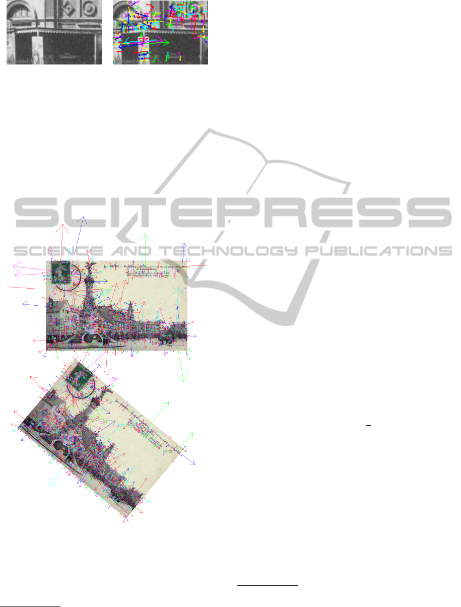
Figure 5: Detected feature points on an image of an old

postcard of the Reims Circus (France).

and on the right the different feature points detected

on with the SIFT algorithm. We mention one more

time many detections at different scales and princi-

pally in the highly contrasted zones. Details in the

images are represented at lower scales, i.e fac¸ade dec-

orative architectural details of the circus. At higher

scales feature points illustrate the spatial organization

of the coarse elements present in the image (openings,

windows....)

Figure 6: Detected feature points on an image of an old

postcard of the Reims Erlon Place (France). On the top the

detected feature points on the original image, on the bottom

the detected feature points on a rotated image.

Figure 6 presents the features detection obtained

on an Reims Erlon Place old postcard

. This ﬁgure

&ref=diversreims/0003.jpg

http://amicarte51.free.fr/reims/carte.php3?itempoint=6

illustrates the features detected on a correctly oriented

image and the ones obtained on a rotated image. We

can observe here that the detected features are similar

in the two images even if some features detected near

the borders are not the same. This is due to the fact

both of the images contain white borders allowing the

rotation (the image submitted to the algorithm must

be rectangular).

4 COMPARISON

It exists many implementations of the SIFT algorithm,

we selected here two of them

. A Matlab executable

implementation is proposed by Lowe on his website

(cf. part 3.) Another implementation computed in

C++ using the OpenCV library for image processing

is provided by Hess

. As we wanted to control the

parameterization of the algorithm, we also computed

our own implementation in C++ using OpenCV. Our

implementation results in this section respect the pa-

rameters suggested by Lowe in 2004.

In this section we will discuss the parameters sug-

gested by Lowe in 2004 analyzing the results we ob-

tain with his executable implementation. We will

compare his results to those obtained with the Hess

implementation and to ours.

4.1 Parametrization of the Algorithm

In section 2 we have described the SIFT algorithm and

the parameters that Lowe recommended after some

empiric tests. In (Lowe, 2004) Lowe suggest to build

a pyramid of three octaves, each of them composed

of ﬁve smoothed images. The smoothing scale fac-

tors increase uniformly with

√

2 frequency between

each image. In theory the highest scale factor that

can be reached on the last image of an octave is

4σ

= 4 ∗1.6 = 6.4. Thereby, at same resolutions,

the largest scale factor σ under which a feature point

can be detected is 6.5 ∗2 = 12.8 at the last image of

the third octave. We analyze the features points ex-

tracted with the implementation of Lowe. We observe

that this value is exceeded. We then conclude that the

Lowe’s implementation increases the number of oc-

taves of the constructed pyramid or the number of im-

ages in each octave comparing to the values suggested

in (Lowe, 2004).

&ref=erlon/0004.jpg

A third interesting one is http://www.vlfeat.org/

overview/sift.html

http://blogs.oregonstate.edu/hess/code/sift/

A COMPREHENSIVE AND COMPARATIVE SURVEY OF THE SIFT ALGORITHM - Feature Detection, Description,

and Characterization

471

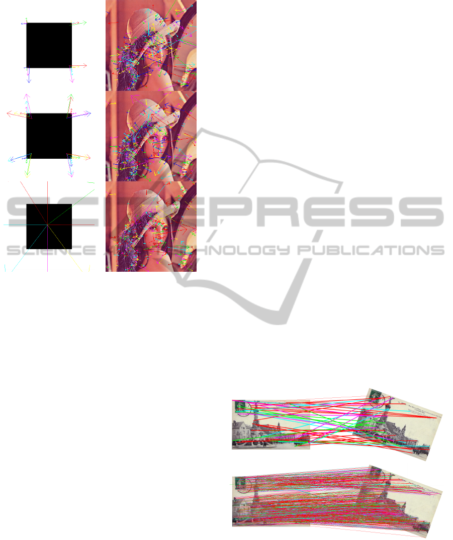
Figure 7: SIFT feature points detection obtained with three

different implementations: our’s (top), Lowe’s (center) and

Hess’s(bottom.)

4.2 Feature Points Validation

In ﬁgure 7 we present feature point detection results

on a synthetic image on the left and Lena image on the

right. The ﬁrst line of this ﬁgure corresponds to the

results we obtained with our implementation of the

algorithm, the middle line with the executable Lowe’s

implementation and ﬁnally the bottom line with the

Hess implementation.

The synthetic image represents a black square

over a white background. We observe that feature

points associated to low scale factors, i.e points with

high curvatures as the square corners, are not detected

by the Hess implementation. Such points are nor-

mally detected in the ﬁrst steps of the process. We

can then conclude that the implementation of Hess do

not consider low scale or that it rejects edge points

of high curvature. We notice that our implementa-

tion detects features with low scale factors. However,

Lowe detects more feature points. They correspond to

higher scales (greater than 12.8). Similarly, the points

detected by Hess represent really high scale features.

The results obtained with Lena’s image shows that

more feature points were detected in highly contrasted

zones. We can notice that the different structures de-

scribed in section 3 are characterized here. An obvi-

ous similarity of the detected features is denoted on

the feather, the details of the hat, the highly curved

architectural structures.... Once more, less feature

points appears within Hess results. The main dis-

similarity between our implementation and the two

other implementations concerns the survey of the high

scales. This study validates the feature points detec-

tion process for the three implementations.

A validation of the quality of the detected feature

point descriptors is fundamental since these are cru-

cial for the matching process.

4.3 Validation of the Descriptors

The robustness of the computed descriptors can be

validated through the matching process. The method

we use to match two different images is the one pro-

posed by Lowe in (Lowe, 2004). For each feature

point in the original image, the Euclidien distance is

computed between the associated descriptor and all

the feature points descriptors present in the second

image. A distance ratio of the two closest neighbors

is then compared to a threshold of 0.6. The closest de-

scriptor is considered as a candidate match if the ratio

do not exceed this threshold. To validate the robust-

ness of the computed descriptors, we test the results

of the matching between an image and its associated

transformed image obtained by a known transforma-

tion. Thus, once a match is found, we compute the

distance between the identiﬁed feature point and the

real match obtained applying the transformation. If

this distance is higher than 3 or 5 pixels, the candi-

date match is rejected.

Figure 8: Matches identiﬁed without rotation of the descrip-

tor (top) and with its rotation (bottom). The thick lines cor-

respond to wrong matches while thin lines represent correct

matches.

This approach proves the importance of the rota-

tion of the descriptor window relatively to the dom-

inant orientation of the feature point as described in

VISAPP 2012 - International Conference on Computer Vision Theory and Applications

472

the section 2.4. Figure 8 shows results of the match-

ing process obtained for the rotated (20

◦

) Reims Erlon

Place postcard. Wrong matches are here represented

by thick lines while thin lines correspond to correct

matches considering a 5 pixels tolerance. The top part

of the ﬁgure was obtained with a static descriptor win-

dow. In this case we notice that few matches were

detected, and that most of them are wrong. The bot-

tom part of the ﬁgure illustrates the results obtained

with a mobile (rotary) descriptor window. In this case

matches are numerous and they are roughly correct.

0 30 60 90 120 150 180 210 240 270 300 330 360

80.0

90.0

100.0

Rotation angle

% of correct match

Lowe04

0 30 60 90 120 150 180 210 240 270 300 330 360

80.0

90.0

100.0

Rotation angle

% of correct match

Lowe

0 30 60 90 120 150 180 210 240 270 300 330 360

80.0

90.0

100.0

Rotation angle

% of correct match

Hess

Figure 9: Percentage of correct matches depending on the

rotation angle of the image. Results are obtained one the

fragment of the Reims Circus old postcard using the three

implementations: our’s (Lowe 2004), Lowe’s and Hess’s.

The dotted line was obtained with a maximal error tolerance

of 3 pixels, the continuous one with a 5 pixels tolerance.

As (Morel and Yu, 2011) have proven the scale-

invariance of the SIFT method, we will focus our

study on invariance to rotation. A series of tests is per-

formed for the two tolerance levels (3 and 5 pixels).

Images are successively rotated by an angle of 10

◦

un-

til reaching 350

◦

. Figure 9 shows the variations of the

percentage of correct matches relatively to the angle

of the rotation, the two levels of distance error tol-

erance and using the three different implementations

of the SIFT algorithm. These results are obtained for

the fragment of the Reims Circus old postcard. The

same tests computed for the Reims Erlon Place old

postcard (presented in Figure 8) show a stable per-

centage of 96% for all the implementations and for

both tolerance levels. In ﬁgure 9 Lowe detected 157

feature points on the original image and obtained a

mean value of 110 matches overall the rotated images

according to the two error tolerances. Hess detected

111 feature points on the original image and obtained

a mean value of 84 matches. We detected 128 fea-

ture points on the original image and obtained a mean

value of 77 matches. In the image of the Reims Erlon

Place, Lowe detected 1973 feature points on the origi-

nal image and obtained a mean value of 1500 matches

according to the 3 pixels error tolerance and 1513 ac-

cording to the 5 pixels one. Hess detected 1463 fea-

ture points on the original image and obtained a mean

value of 1004 matches according to the 3 pixels er-

ror tolerance and 1016 according to the 5 pixels one.

We detected 1510 feature points on the original image

and obtained a mean value of 937 matches accord-

ing to the two error tolerances. We can notice that on

these two ﬁgures that the results are obviously very

performing when the error tolerance is of 5 pixels for

both images and the three implementations. When the

error tolerance is of 3 pixels, the results are preform-

ing and comparable for the Reims Erlon Place old

postcard. We notice a lower performance for the frag-

ment of the Reims Circus old postcard. Even if Hess

found more matches in this case than us, his imple-

mentation presents the worst results cause he detected

more wrong matches, the Lowe’s one is the best even

if for some angles our implementation parametrized

according to Lowe 2004 shows better matching per-

centage.

Reims Circus Erlon Place

3 px 5 px 3 px 5 px

Lowe04 95.05 99.56 97.64 99.41

Lowe 96.87 99.26 99.41 99.96

Hess 89.65 98.23 97.86 99.23

Figure 10: Evaluation of the matching process on the Reims

Circus postcard extract and the Reims Erlon Place postcard

for 3 and 5 pixels tolerance levels.

Figure 10 presents the means percentage of cor-

rect matches for all the angles of rotation for both

levels of tolerance computed for the fragment of the

Reims Circus old postcard and the Reims Erlon Place

old postcard. The three aforementioned implemen-

tations where tested: our (Lowe04) implementation,

Lowe’s executable Matlab implementation and Hess’s

implementation. We notice performing results for all

the implementation with an advantage for the Lowe’s

implementation. Our results are situated between the

Hess’s and Lowe’s while being dependent of the test

image.

5 CONCLUSIONS

In this paper, we presented a synthetic view of the

SIFT algorithm insisting on the tricky steps of its im-

plementation. We analyzed and discussed the prop-

erties of the detected feature points and their corre-

A COMPREHENSIVE AND COMPARATIVE SURVEY OF THE SIFT ALGORITHM - Feature Detection, Description,

and Characterization

473

sponding descriptors. We presented a survey of three

implementations of the algorithm: Lowe’s, Hess’s

and our’s implementation respecting the parametriza-

tion suggested by Lowe in 2004. We studied the dif-

ferences between these implementation and conclude

on the robustness of all of them with an advantage

for the Lowe’s implementation. Our implementation

will be used in the context of the spatio temporal 3-

D reconstruction of the city of Reims using old post-

cards as data. The challenge is to take into account

the architectural evolution across the years in order to

match the different views of the buildings.

REFERENCES

Bay, H., Ess, A., Tuytelaars, T., and Van Gool, L. (2008).

Speeded-up robust features (surf). Computer Vision

and Image Understanding, 110(3):346–359.

Harris, C. and Stephens, M. (1988). A combined corner and

edge detector. In Alvey Vision Conf., pages 147–151.

Manchester, UK.

Juan, L. and Gwun, O. (2009). A comparison of sift, pca-sift

and surf. Int. Journal of Image Processing, IJIP’09,

3(4):187–152.

Ke, Y. and Sukthankar, R. (2004). Pca-sift: A more distinc-

tive representation for local image descriptors. Com-

puter Society Conf. on Computer Vision and Pattern

Recognition , CVPR’04, 2:506–513.

Lowe, D. (2004). Distinctive image features from scale-

invariant keypoints. Int. Journal of Computer Vision,

60(2):91–110.

Mikolajczyk, K. and Schmid, C. (2005). A performance

evaluation of local descriptors. IEEE trans. on Pat-

tern Analysis and Machine Intelligence, 27(10):1615–

1630.

Morel, J. and Yu, G. (2011). Is sift scale invariant? Inverse

Problems and Imaging, 5(1):115–136.

Smith, S. and Brady, J. (1997). Susan a new approach to

low level image processing. Int. Journal of Computer

Vision, 23(1):45–78.

VISAPP 2012 - International Conference on Computer Vision Theory and Applications

474