
ON STOCHASTIC TREE DISTANCES AND THEIR TRAINING VIA
EXPECTATION-MAXIMISATION
Martin Emms
School of Computer Science and Statistics, Trinity College, Dublin, Ireland
mtemms@tcd.ie
Keywords:
Tree-distance, Expecation-Maximisation.
Abstract:
Continuing a line of work initiated in (Boyer et al., 2007), the generalisation of stochastic string distance to
a stochastic tree distance is considered. We point out some hitherto overlooked necessary modifications to
the Zhang/Shasha tree-distance algorithm for all-paths and viterbi variants of this stochastic tree distance. A
strategy towards an EM cost-adaptation algorithm for the all-paths distance which was suggested by (Boyer
et al., 2007) is shown to overlook necessary ancestry preservation constraints, and an alternative EM cost-
adaptation algorithm for the Viterbi variant is proposed. Experiments are reported on in which a distance-
weighted kNN categorisation algorithm is applied to a corpus of categorised tree structures. We show that a
67.7% base-line using standard unit-costs can be improved to 72.5% by the EM cost adaptation algorithm.
1 INTRODUCTION
The classification of tree structures into cate-
gories is necessary in many settings. In natu-
ral language processing an example is furnished by
Question-Answering systems, which frequently have
a Question-Categorisation sub-component, whose
purpose is to assign the question to one of a number of
predefined semantic categories (section 5 gives some
details). Often one would like to obtain such a clas-
sifier by a data-driven machine-learning approach,
rather than by hand-crafting one. The distance-
based approach to such a classifier is to have a pre-
categorised example set and to compute a category
for a test item based on its distances to examples in
the example set, such as via k-NN.
With items to be categorised represented as trees,
a crucial component in such a classifer is the mea-
sure used to compare trees. The tree-distance first
proposed by (Tai, 1979) is a well motivated candidate
measure (see later for further details). This measure
can be seen as composing a relation between trees out
of several kinds of atomic operations (match, swap,
delete, insert) the costs of which are dependent on the
labels of the nodes involved. The performance of such
a distance-based classifier is therefore very dependent
on the settings of these atomic costs.
In the work presented below probabilistic variants
of the standard tree-distance are considered and then
Expectation-Maximisation techniques are considered
as potential means to adapt atomic costs given a cor-
pus of training tree pairs.
Section 2 recalls the standard definitions of string-
and tree-distance. Section 3 goes on to first recall the
stochastic string-distance as proposed by (Ristad and
Yianilos, 1998) and then defines stochastic variants of
tree-distance, which we term All-scripts and Viterbi-
script stochastic Tai distances D
a
s
(S,T) and D
v
s
(S,T).
The standard algorithm of (Zhang and Shasha, 1989)
for the tree-distance is then recalled and some nec-
essary modifications to allow correct and efficient
computation of the All-scripts and Viterbi variants
are described. Section 4 concerns how one might
adapt atomic costs from a training corpus of same-
category neighbours via Expectation-Maximisation.
The string-case is recalled and then a brute-force, ex-
ponentially expensivemethod for adapting the param-
eters of the All-scripts distance is outlined. Whilst for
the linear case, a particular factorisation is applica-
ble which permits efficient implementation of the EM
all-scripts method, we show by means of a counter-
example that for the tree case this kind of factori-
sation is not applicable, although it has been sug-
gested in (Boyer et al., 2007) that it is. This leads
to a proposed method for adapting the parameters of
the Viterbi-script distance, something which is feasi-
ble. Section 5 then reports some experimental out-
comes obtained with this EM procedure for adapting
the Viterbi-script distance.
Emms M. (2012).
ON STOCHASTIC TREE DISTANCES AND THEIR TRAINING VIA EXPECTATION-MAXIMISATION.
In Proceedings of the 1st International Conference on Pattern Recognition Applications and Methods, pages 144-153
DOI: 10.5220/0003864901440153
Copyright
c
SciTePress

2 NON-STOCHASTIC SEQUENCE
AND TREE DISTANCES
Let us begin by formulating some definition relation
to the familiar notion of string-distance. The formu-
lations follow closely those of (Ristad and Yianilos,
1998) and are chosen to allow an easy transition to
the stochastic case.
Let S be an alphabet. Let the set of edit operation
identifiers, EdOp, be defined by
EdOp = ((S ∪{l } ) × (S ∪ {l }))\hl ,l i
and let an edit-script be a sequence e
1
...e
n
#, n ≥ 0,
with each e
i
∈ EdOp and with # as a special end-of-
script marker. Given an edit-script A , it can be pro-
jected into a ’source’ string src(A ) ∈ S
∗
, by contenat-
ing the left elements of the contained operations, and
likewise into a ’target’ string trg(A ) ∈ S
∗
:
src(#) = e trg(#) = e
src(hl ,yiA ) = src(A ) trg(hx,l iA ) = trg(A )
src(hx,yiA ) = x src(A ) trg(hx,yiA ) = y trg(A )
The yield of edit-script A can be defined as pair
of strings hsrc(A ),trg(A )i. If (s,t) = yield(A ), each
e
i
∈ A is interpretable as an edit operation in a process
of transforming s to t: deletion (a,l ), insertion (l , b),
or match/substitution (a, b). Let E(s,t) be all scripts
which yield (s,t). The multiple scripts in E(s,t) de-
scribe alternative ways to transform s into t.
If costs are defined for such edit-scripts, a string-
distance between s and t can be defined as the cost of
the least-cost script in E(s,t).
Alternatively one can consider the partial, 1-to-
1, order-respecting mappings from s to t. Costs can
be defined for such mappings and a distance mea-
sure defined via minimising these costs. Script-based
and mapping-based definitions are equivalent (Wag-
ner and Fischer, 1974): fundamentally an edit-script
is viewable as a particular serialisation of a mapping.
For ordered, labelled trees, the analogue to stan-
dard string distance was first considered by (Tai,
1979). We develop the definitions relevant to this
below, starting first with a mapping-based definition.
The equivalent script-based definition follows this.
A Tai mapping is a partial, 1-to-1 mapping s from
the nodes of source tree S to a target tree T which re-
spects left-to-right order and ancestry
1
. For the pur-
pose of assigning a score to such a mapping it is con-
venient to identify three sets:
1
So if (i
1
, j
1
) and (i
2
, j
2
) are in the mapping, then (T1)
le ft(i
1
,i
2
) iffle ft( j
1
, j
2
) and (T2) anc(i
1
,i
2
) iff anc( j
1
, j
2
)
M the (i, j) ∈ s : the ’matches’ and ’swaps’
D the i ∈ S s.t. ∀ j ∈ T,(i, j) 6∈ s : the ’deletions’
I the j ∈ T s.t. ∀i ∈ S,(i, j) 6∈ s : the ’insertions’
Where S is the label alphabets of source and target
trees, let g (i) be the label of node i. Let C be a cost
table of dimensions |S | + 1 × |S | + 1. The cost of a
mapping is the sum over the atomic costs defined by
2
for (i, j) ∈ M cost is C [g (i)][g ( j)]
for i ∈ D cost is C [g (i)][0]
for j ∈ I cost is C [0][g ( j)]
The so-called unit-cost matrix, C
01
has 0 on the diag-
onal and 1 everywhere else. For a given cost matrix
C , the Tai- or tree-distance D (S,T) is defined as the
cost of the least-costly Tai mapping s between S and
T.
There is an alternative, more procedural definition
route, via tree-edit operations analogous to string-edit
operations. The table below depicts the three edit op-
erations:
operation script element
x
(m
~
l (x
~
d)~r)
→ (m
~
l
~
d~r)
(x,l )
y
(m
~
l
~
d~r)
→ (m
~
l (y
~
d)~r)
(l ,y)
x y
(m
~
l (x
~
d)~r)
→ (m
~
l (y
~
d)~r)
(x,y)
Thus deletion involves making the daughters of some
node x into the daughters of that node’s parent m,
insertion involves taking some of the daughers of a
node m and making them instead the daughters of a
newdaughter y of m, and swapping/matching involves
simply replacing some node x with a node y at the
same position.
The right-hand column shows the script element
which is used to record the use of particular edit op-
eration. Using the same table of cost C as was used
for costing a mapping, a cost can be assigned to the
script describing the operations to transform a tree S
into a tree T, and a script-based definition of distance
then given via minimising this cost.
The mapping- and script-based definitions are
equivalent (Tai, 1979; Kuboyama, 2007), with a script
serving as a serialised representation of a mapping.
(Zhang and Shasha, 1989) provided an efficient algo-
rithm for its calculation.
2
See also (Emms and Franco-Penya, 2011) in these pro-
ceedings.

To illustrate, below is shown first a mapping be-
tween two trees, and second the sequence of edit-
operations corresponding to it, with some of the inter-
mediate stages as these operations are applied; with
unit-costs the distance is 3
3
:
a
a
ba b
b
c
a b
b
a
b
a
a
ba b
b
c
a b
b
a
b
a b
b
a
b
a
(b,b)(a,a)(b,b)(.,a)
(b,b)(a,.)
(a,c)
a
a
a b
b b
a
It is easy to see that for strings encoded as linear,
vertical trees, the string-distance and tree-distance co-
incide. We will use tree-distance and Tai-distance in-
terchangeably, though the literature contains several
other, non-equivalent notions bearing the name tree-
distance. Based, as it is, simply on the notion of map-
pings respecting the two defining dimensions of trees,
the Tai distance seems a particularly compelling no-
tion.
3 STOCHASTIC SEQUENCE AND
TREE DISTANCES
(Ristad and Yianilos, 1998) introduced a probabilis-
tic perspective on string distance, defining a model
which assigns a probability to every possible edit-
script. Edit-script compoments e
i
∈ EdOp∪ {#} are
pictured as generated in succession, independently of
each other. There is an emission probability p on edit-
script components, such that
å
e∈EdOp∪{#}
p(e) = 1,
and a script’s probability is defined by
P(e
1
... e
n
) =
Õ
i
p(e
i
)
For a given string pair (s,t), as before E(s,t) de-
notes all the edit-scripts which have (s,t) as their
3
It is worth noting that for the equivalence between
mapping-based costs and script-based costs, the scripts
which correspond to mappings mention each source and tar-
get symbol exactly once. Thus the ’short’ script segments
shown in the picture are not representative of the scripts
which correspond to a mapping
yield. They then define the all-paths stochastic edit
distance, P
a
(s,t), as the sum of the probabilities of all
scripts e ∈ E(s,t), whilst the viterbi version P
v
(s,t) is
the probability of the most probable one.
It is natural to consider to what extent the proba-
bilistic perspectiveadopted for string-distance by Ris-
tad and Yianilos can be applied to tree-distance. The
simplest possibility is to use exactly the same model
of edit-script probability, which leads to the notions:
Definition 1 (All-scripts stochastic Tai similari-
ty/distance). The all-scripts stochastic Tai similarity,
Q
A
s
(S,T), is the sum of the probabilities of all edit-
scripts which represent a Tai-mapping from S to T.
The all-scripts stochastic Tai distance, D
A
s
(S,T), is its
negated logarithm, ie.
2
−D
A
s
(S,T)
= Q
A
s
(S,T)
Definition 2 (Viterbi-script stochastic Tai similari-
ty/distance). The Viterbi-script stochastic Tai similar-
ity, Q
V
s
(S,T), is the probability of the most proba-
ble edit-script which represents a Tai-mapping from
S to T. The Viterbi-script stochastic Tai distance,
D
V
s
(S,T), is its negated logarithm, ie.
2
−D
V
s
(S,T)
= Q
V
s
(S,T)
For Q
A
s
and Q
V
s
the probabilities on each possi-
ble component of an edit script, EdOp ∪ {#}, must
be defined. In a similar fashion to the non-stochastic
case, let this be defined by a table C
Q
of dimensions
|S | + 1 × |S | + 1 such that:
for hx,yi ∈ S × S p(hx,yi) = C
Q
(x,y)
for x ∈ S p(hx,l i) = C
Q
(g (i),0)
for y ∈ S p(hl , yi) = C
Q
(0,g ( j))
p(#) = C
Q
(0,0)
For convenience C
Q
(0,0) is interpreted as p(#). The
sum over all the entries in this table should be 1. It
is clear that an equivalent cost-table C
D
can be de-
fined, containing the negated logs of the C
Q
entries,
and that D
V
s
(S,T) can be equivalently defined by an
additive scoring of the scripts using the entries in C
D
.
Therefore D
V
s
(S,T) coincides with the standard no-
tion of tree-distance
4
if the cost-table is restricted to
be the image of a possible probability-table under the
negated logarithm mapping. We will call such tables
stochastically valid cost tables. Again it is easy to see
that with sequences encoded as vertical trees, these
notions coincide with those defined on sequences by
Ristad and Yianilos.
4
D
V
s
(S,T) will include a contribution from the negated
log of p(#). As all pairs will share this contribution, any
application ranking pairs can ignore this contribution.

For the Viterb-script distance D
V
s
(S,T), the well
known Zhang/Shasha algorithm is an implementa-
tion. The Viterbi-script similarity Q
V
s
can also be ob-
tained by a variant replacing + with ×. Implementing
the All-script distance D
A
s
(S,T) (or equivalent simi-
larity Q
A
s
(S,T)) turns out though to require one sub-
tle change to the original Zhang/Shasha formulation.
This is explained at further length below.
Figure 1 gives an algorithm for D
A
s
and D
V
s
. To dis-
cuss it first some definitions from (Zhang and Shasha,
1989) are required. The algorithm operates on the
left-to-right post-order traversals of trees. If k is the
index of a node of the tree, the left-most leaf, l(k), is
the index of the leaf reached by following the left-
branch down. For a given leaf there is a highest
node of which it is the left-most leaf and any such
node is called a key-root. For any tree S, KR(S) is
the key-roots ordered by position in the post-order
traversal. If i is the index of a node of S, S[i] is the
sub-tree of S rooted at i (i.e. all nodes n such that
l(i) ≤ n ≤ i). Where i is any node of a tree S, for
any i
s
with l(i) ≤ i
s
≤ i, the prefix of S[i] from l(i) to
i
s
can be seen as a forest of subtrees of S[i], denoted
For(l(i),i
s
).
The description instantiates to two algorithms,
with x = V for Viterbi, and x = A for All-Scripts.
In both cases, it is a doubly nested loop ascending
through the key-roots of S and T, in which for each
pair of key-roots (i, j), a sub-routine tree dist
x
(i, j) is
called. Values in a tree-table T are set during calls to
tree dist
x
(i, j) and persist. Each call totree dist
x
(i, j)
operates on a sub-region
5
of the forest-table F , from
l(i) − 1,l( j) − 1 to i, j. The loop is designed so that
F [i
s
][ j
t
] is the forest-distance from For(l(i), i
s
) to
For(l( j), j
t
). F -entries do not persist between sep-
arate calls to tree dist
x
(i, j).
In the Viterbi case, TD
V
, there is no inversion
from neg-logs to probabilities, and the algorithm can
be applied when C
D
is an arbitrary table of atomic
costs.
It is the design of case 2 that enforces that only
Tai mappings are considered: when a forest distance
F
V
[i
s
][ j
t
] is to be computed, the possibility that i
s
is
mapped to j
t
is factored into a forest+tree combina-
tion TM
V
= F
V
[l(i
s
) − 1][l( j
t
) − 1] + T
V
[i
s
][ j
t
], so
that descendants of i
s
can only possibly match with
descendants of j
t
and vice-versa.
Setting x to V for Viterbi, the algorithm is almost
identical to that in (Zhang and Shasha, 1989), except
5
The initialisation sets the left-most column of this to
represent the pure deletion cases For(l(i), i
s
) to
/
0, and the
uppermost row to represent the pure insertion cases
/
0 to
For(l( j), j
t
)
input:
traversals S and T of two trees
a cost table C
D
compute KR(S), KR(T)
create table T
x
, size | S | × | T |
create table F
x
, size | S | + 1 × | T | + 1
TD
x
(S,T) {
for each i ∈ KR(S) in ascending order {
for each j ∈ KR(T) in ascending order {
execute tree dist
x
(i, j)}
}
return
F
x
[|S|][|T|]
}
tree dist
x
(i, j) {
where
i
0
= l(i) − 1, j
0
= l( j) − 1
F
x
[i
0
][ j
0
] = 0 initialize
for
i
s
= l(i)
to
i
s
= i {
F
x
[i
s
][ j
0
] = F
x
[i
s
− 1][ j
0
] +C
D
(g (i
s
),0) }
for
j
t
= l( j)
to
j
t
= j {
F
x
[i
0
][ j
t
] = F
x
[i
0
][ j
t
− 1] +C
D
(0,g ( j
t
)) }
for
i
s
= l(i)
to
i
s
= i
for
j
t
= l( j)
to
j
t
= j loop
M
x
= F
x
[i
s
− 1][ j
t
− 1] +C
D
(g (i
s
),g ( j
t
))
D
x
= F
x
[i
s
− 1][ j
t
] + C
D
(g (i
s
),0)
I
x
= F
x
[i
s
][ j
t
− 1] + C
D
(0,g ( j
t
))
TM
x
= F
x
[l(i
s
) − 1][l( j
t
) − 1]+T
x
[i
s
][ j
t
]
1
:if(
l(i
s
) == l(i)
and
l( j
t
) == l( j)
)
{
F
x
[i
s
][ j
t
] = OP
x
(M
x
,D
x
,I
x
)
T
x
[i
s
][ j
t
] = M
x
(∗)}
2
:if(
l(i
s
) 6= l(i)
or
l( j
t
) 6= l( j)
)
{F
x
[i
s
][ j
t
] = OP
x
(D
x
,I
x
,TM
x
)}
Figure 1: Viterbi and All-paths tree-distance algorithms.
Set x to V throughout for Viterbi, with OP
V
= min,
and x to A for All-paths, with OP
A
= logsum, where
logsum(x
1
.. .x
n
) = −log(
å
i
(2
−x
i
)).
for the asterixed line, which in the original would be:
T
V
[i
s
][ j
t
] = F
V
[i
s
][ j
t
](∗∗)
Whereas the original (**) formula for updating the
tree table in case 1 updates it to store the true tree-
distance between S[i
s
] and T[ j
t
], the (*) variant stores
just M
V
, the cost of the least-cost script for an align-
ment of For(l(i
s
),i
s
) to For(l( j
t
), j
t
) in which nodes
i
s
and j
t
are mapped to each other. For the Viterbi
cost, (*) and (**) could be interchanged and so have
T
V
[i
s
][ j
t
] store a cost in which i
s
and j
t
might not be
mapped to each other: in such a case when the values
in T
V
are called on in case 2, the TM
V
component
will just be equal to one or other of the I
V
or D
V
com-
ponents over which the minimum is calculated.
Reading the algorithm now with x set to A, T
A
and
F
A
represent the ’all-scripts’ probabilities, sums over
all scripts which serialize a Tai mapping between the
relevant trees or forests. Looking again at the aster-

ixed line, through not setting T
A
[i
s
][ j
t
] = F
A
[i
s
][ j
t
],
T
A
[i
s
][ j
t
] is not the log of the sum of the probabilities
of all the scripts which can align S[i
s
] and T[ j
t
] but in-
stead the sum over all the cases in which i
s
is mapped
to j
t
. For the subsequent use of T
A
in case 2, this is
now a necessary feature: if T
A
[i
s
][ j
t
] does not have
this interpretation then when these values are called
upon in case 2, probabilities of scripts ending in either
deletion of i
s
or insertion of j
t
are doubly counted.
Example. Let t
1
= t
2
= (b (b) (a b)), and suppose
the cost-table to the right below, which represents as
negated logs the assumptions that all probabilites are
0 except for p(a,l ) = 1/8 = p(l ,a), p(b, b) = 1/4,
and p(#) = 1/2. The left is the only Tai-mapping
which is associated with a non-zero probability edit-
script in this setting
b
b
b
b
a
b
a
b
l a b
l 1 3 inf
a 3 inf inf
b inf inf 2
By inspection, Q
A
s
(t
1
,t
2
) = (1/2)
6
(1/64),
Q
V
s
(t
1
,t
2
) = (1/2)
6
(1/128), and these are the
values, or rather their negated logs, which will be
calculated
6
by the algorithm in Figure 1. However,
if T
A
[a
3
][a
3
] were to include the probabilities for
scripts involving the deletions or insertions of a,
Q
A
s
(t
1
,t
2
) would be incorrectly calculated to be
(1/2)
6
(3/64).
As a final remark concerning the algorithm for the
Viterbi case, it is straightforward to extend the algo-
rithm so that it returns not just the cost of the best
script but also the best script itself. Hence we shall
write (v,V) = TD
V
(S,T).
4 EM FOR COST ADAPTATION
As noted in section 1, a possible use of a distance
measure is for deployment in a k-NN classifier, deter-
mining a category for a test item based on its distances
to examples in a pre-categorised example set. This is
the case in the experiments reported on in section 5.
In those experiments the categorised items are the
syntax-structures of natural language questions, and
the categories are broad semantic categories, such as
HUM
(’the question expects a human being to be iden-
tified as the answer’) or
LOC
(’the question expects a
6
The reason for the premultiplying (1/2)
6
factor in these
numbers is that it is easier in this case to calculate first ig-
noring p(#) and from a table in which all entries are twice
as large, and thento correct for the over-estimation; the only
scripts making any contribution all have length 5
location to be identified as the answer’).
For the tree-distance measures, the performance
of the classifier is going to vary with the atomic pa-
rameter settings in the cost-table C
D
. One might ex-
pect that scripts between pairs of trees (or strings)
that belong to the same category differ from scripts
between pairs of trees (or strings) that belong to dif-
ferent categories. For example, for the question-
categorisation scenario, on same-category pairs one
might expect that the substitution (who/when) to
be less frequent that the substitution state/country.
In terms of the parameters of the stochastic dis-
tances this would correspond to P(who,when) <<
P(state,country), or equivalently in terms of negated
logs, C
D
(who,when) >> C
D
(state,country). This
leads to the idea that one might be able to use
Expectation-Maximisation techniques (Dempster et
al., 1977) to adapt edit-probs from a corpus of same-
category nearest neighbours.
adaptation
EM
of costs
nearest
same−category
neighbours
Such a technique, for the case of stochastic string
distance, was first proposed by (Ristad and Yianilos,
1998).
4.1 All-scripts EM
As a first step towards a cost-adaptation algorithm,
consider the following brute-force all-scripts EM al-
gorithm, EM
A
bf
, consisting in interations of the fol-
lowing pair of steps
(Exp)
A
generate a virtual corpus of scripts by treat-
ing each training pair (S,T) as standing for all the
edit-scripts s , which can relate S to T, weighting
each by its conditional probability P(s /Q
A
s
(S,T),
under current probalities C
Q
(Max) apply maximum likelihood estimation to the
virtual corpus to derive a new probability table.
A virtual count or expectation g
S,T
(op) contributed by
S, T for an operaton op can be defined by
g
S,T
(op) =
å
s :S7→T
[
P(s )
Q
A
s
(S,T)
× freq(op ∈ s )]
and the (Exp)
A
accumulating these values g
S,T
(op)
for all possible op’s over all training pairs. The pic-
ture below attempts to illustrate this for a particular

operation (a,l ) occuring in various scripts between a
particular tree pair
a
a b
b b
a
c
b
b
b
aa
s
i
)P(
A
=S
s
1
s
i
s
n
= occ. of (a,.)
(a,.)
b
b
b
a
a
a
a b
b b
a
Q
For the case of linear trees, this amounts to the same
adaptation proposal as that put forward by (Ristad
and Yianilos, 1998). This brute-force algorithm is
exponentially expensive. To obtain a feasible equiv-
alent algorithm one may attempt to apply the same
strategy as that used by (Ristad and Yianilos, 1998)
for the case of linear trees, which is for each tree
pair (S,T), to first compute position-dependent ex-
pectations g
(S,T)
[i][ j](op) for each operation and then
sum these position-independent expectations to give
the expecations per-pair g
(S,T)
(op). In this approach,
g
(S,T)
[i][ j](m,m
′
), the expectation for a swap (m, m
′
)
at (i, j) has the semantics
g
(S,T)
[i, j](m,m
′
) =
å
s ∈E(S,T ),(m
i
,m
′
j
)∈s
[
p(s )
Q
A
s
(S,T)
]
=
1
Q
A
s
(S,T)
×
å
s ∈E(S,T),(m
i
,m
′
j
)∈s
[p(s )]
or in words, it is the sum over the conditional prob-
abilities of any script s containing a m
i
,m
′
j
substitu-
tion, given that it is a script between S and T.
For the case of linear trees, the position-
dependent expectations g
(S,T)
[i][ j] can be computed
feasibly because firstly, the summation in the above
can be factorised into a product of 3 terms
å
s ∈E(S,T),(m
i
,m
′
j
)∈s
[p(s )]
=
å
s
pre
∈E(S
1:1−1
,T
1:j−1
)
[p(s
pre
)]×
p(m,m
′
)×
å
s
suf f
∈E(S
i+1:I
,T
j+1:J
)
[p(s
suf f
)]
(1)
and secondly the summations over the possible scripts
prefixing (m
i
,m
′
j
), and the possible scripts suffixing
(m
i
,m
′
j
) can be straightforwardly calculated; the first
is the all-scripts algorithm, and the second an easily
formulated ’backwards’ variant.
For the case of general trees (as opposed to linear
trees) (Boyer et al., 2007) propose such a factorisa-
tion approach. Their proposal turns out, however, to
be unsound, factorizing the problem in a way which
is invalid giventhe ancestry-preservationaspect of Tai
mappings
7
. To explain this, consider Figure 2, which
reproduces the essentials of an example from their pa-
per
8
.
7
A fact which they concede p.c.
8
Fig. 3 p61
1
7
2
6
3 5
6
1
4
5
2 3
4
m
m’
(i)
(ii)
(iii)
Figure 2: The swap-case in expectation calculation.
For the pair of trees, we wish to calculate the position-
dependent expectation g [4,4](m,m
′
). (Boyer et al.,
2007) propose an algorithm implying the correctness
of the factorisation
å
s ∈E(S,T),(m
4
,m
′
4
)∈s
[p(s )]
=
å
s
1
∈E([(·
1
)],(·
2
(·
1
)))
[p(s
1
)]× [(i)]
å
s
2
∈E([(·
2
)(·
3
)],[(·
3
)])
[p(s
2
)] × p(m,m
′
) [(ii)]
å
s
3
∈E([(·
6
(·
5
))],[(·
7
(·
6
(·
5
)))])
[p(s
3
)] [(iii)]
(2)
where the terms (i)–(iii) corresponds to the indicated
regions in Figure 2. The problem is with final term
(iii) in the product. Each edit-script s ∈ E(S, T) rep-
resents a Tai mapping between S and T. The summa-
tion
å
s ∈E(S,T),(m
4
,m
′
4
)∈s
[p(s )] refers to those scripts
which represent a Tai mapping with the property that
m
4
is mapped to m
′
4
. This means that if an ances-
tor of m
4
is in the mapping (ie. not deleted) then
its image under the mapping must be an ancestor of
m
′
4
, and vice-versa. The final term in the product,
å
s
3
∈E([·
6
(·
5
)],[·
7
(·
6
(·
5
))])
[p(s
3
)], sums over any script
between these two sub-trees of S and T and this will
include scripts in which node ·
6
of S is mapped to ·
6
of T, and this corresponds to a mapping in which an
ancestor of m
4
is mapped to a non-ancestor of m
′
4
:
1
7
2
6
3 5
6
1
4
5
2 3
4
m
m’
For example if the only non-zero probability script
from (·
6
(·
5
)) to (·
7
(·
6
(·
5
))) is one mapping the ·
6
of
S to the ·
6
of T then g [4, 4](m,m
′
) should be zero,
though according to (2) it will not be.
For general trees, a feasible equivalent to the
brute-force EM
bf
A
remains an unsolved problem.
4.2 Viterbi EM
An approximation to the the All-scripts proposal con-
sists in simply in replacing the Exp
A
step by

(Exp)
V
generate a virtual corpus of scripts by treat-
ing each training pair (S,T) as standing for
the best edit-script s , which can relate S to
T, weighting it by its conditional probability
P(s )/Q
A
s
(S,T), under current costs C
Where V is the best-script, the virtual count or expec-
tation g
S,T
(op) contributedby S, T for the operaton op
would in this case be defined by
g
(S,T)
(op) =
Q
V
s
(S,T)
Q
A
s
(S,T)
× freq(op ∈ V )
and the (Exp)
V
step accumulates these values
g
(S,T)
(op) for all possible op’s over all training pairs.
The picture below attempts to illustrate this for a par-
ticular operation (a, l ) occuring on the best-path V
between a particular tree pair
a
a b
b b
a
c
b
b
b
aa
V)P(
i
(a,.)
b
b
b
a
a
a
a b
b b
a
V
V
=
= occ. of (a,.)
on best−path V
s
i
)P(
A
=SQ
Q
Figure 3 spells out this Viterbi cost-adaptation algo-
rithm for stochastic tree-distance.
9
input:
a set P of tree pairs (S,T)
a cost table C, size |S | + 1 × |S | + 1
create tables g ,C
new
same size as C
while(
conv 6= true
)
{
zero all entries in g
for each
(S,T) ∈ P {
let
(v, V ) = TD
V
(S,T), a = TD
A
(S,T)
g [l ][l ]
+=
2
−v
/2
−a
for each
(x,y) ∈ EdOp {
g [x][y]
+=
( freq o f (x, y) in V ) × 2
−v
/2
−a
}
}
C
new
= −log(g /sum(g ))
if
(C
new
6= C){C = C
new
} else {conv = true}
}
return
C
Figure 3: Viterbi EM cost adaptation for tree-distance. Note
S is the label alphabet of the tree-pairs in P . The algorithms
TD
V
and TD
A
are as defined in Figure 1.
Such Viterbi training variants have been found
beneficial, for example in the context of parameter
training for PCFGs (Bened´ı and S´anchez, 2005).
9
Simple modifications of the algorithm as formulated
force it to generate a symmetric expectation table g .
5 EXPERIMENTS WITH VITERBI
EM COST-ADAPTATION
We have conducted some experiments with this
Viterbi EM cost-adaptation approach. In particular
we have considered how it might adapt a tree-distance
measure that is put to work in a k-NN classification
algorithm.
Figure 4 outline the distance-weighted kNN clas-
sification algorithm which was used in the experi-
ments.
knn class(
Examples,C
D
,k
;T)
{
let D = SORT({(S,D
V
s
(S,T)) | S ∈ Examples }
while(!resolved)
{
P = top(k, D ), V = weighting( P )
if(
no winner in V
)
{
set k = k + 1
}
else
{
resolved = true
}
}
return
category with highest vote in V
}
Figure 4: Distance-weighted k nearest neighbour classifica-
tion.
top(k,D ) basically picks the first k items from D
10
.
The weighting converts the panel of distance-rated
items to weighted votes for their categories, and in the
experiments reported later, the options for the con-
version of an item of category C, at distance d, into
a vote vote(C,d) are Majority: vote(C, d) = 1; Du-
dani: vote(C, d) = (d
max
− d)/(d
max
− d
min
), or 1 if
d
max
= d
min
, where d
max
and d
min
are maximum and
minimum distances in the panel (Dudani, 1976).
It can arise that the test tree T contains a symbol
for which C
D
has no entry. One option is to assign
all operations involving the symbol some default cost
k . See the Appendix for a proof that the ordering of
neigbours is independent of the value chosen for k
In applying the EM
V
cost-adaptation in the con-
text of the k-NN classification algorithm, the training
set for cost-adaptation was taken to consists of tree
pairs (S,T), where for each example-set tree S, T is a
nearest same-category neighbour. The training algo-
rithm should less the stochastic tree-distance between
these trees.
EM
V
like all other EM algorithms needs an ini-
tialisation of its parameters. We will use C
D
u
(d) for
a ’uniform’ initialisation with diagonal factor d. This
will mean that C
D
u
(d) is a stochastically valid cost-
table, with the additional properties that (i) all diag-
onal entries are equal (ii) all non-diagonal entries are
equal (iii) diagonal entries are d times more probable
10
Modulo some niceties concerning ties which space pre-
cludes detailing
than non-diagonal. For these purposes the cost-table
entry for p(#) is treated as non-diagonal. As an illus-
tration, for an alphabet of just 2 symbols, the initiali-
sations C
D
u
(d) for d = 3, 10, 100, and 1000 are:
3 l a b
l 3.7 3.7 3.7
a 3.7 2.115 3.7
b 3.7 3.7 2.115
10 l a b
l 4.755 4.755 4.755
a 4.755 1.433 4.755
b 4.755 4.755 1.433
100 l a b
l 7.693 7.693 7.693
a 7.693 1.05 7.693
b 7.693 7.693 1.05
1000 l a b
l 10.97 10.97 10.97
a 10.97 1.005 10.97
b 10.97 10.97 1.005
As a smoothing option concerning a table C
D
de-
rived by EM
V
, let C
D
l
be its interpolation with the
original C
D
u
(d) as follows
2
−C
D
l
[x][y]
= l (2
−C
D
[x][y]
) + (1− l )(2
−C
D
u
(d)[x][y]
)
with 0 ≤ l ≤ 1, with l = 1 giving all the weight to the
derived table, and l = 0 giving all the weight to the
initial table.
The dataset used was a natural language process-
ing one, being a corpus of (broadly) semantically cat-
egorised, and syntactically analysed questions, which
was created by from two pre-existing datasets. Ques-
tionBank (QB) is a hand-corrected treebank for ques-
tions (Judge et al., 2006; Judge, 2006b), (Judge,
2006a). A substantical percentage of the questions
in QB are taken from a corpus of semantically cat-
egorised, syntactically unannotated questions (CCG,
2001). From these two corpora we created a corpus
of 2755 semantically categorised, syntactically anal-
ysed questions, spread over the semantic categories as
follows
11
Cat HUM ENTY DESC NUM LOC ABBR
N 647 621 533 461 455 38
% 23.48 22.54 19.35 16.73 16.52 1.38
For further details of the software and data see
(Emms, 2011). Figure 5 shows some results of a
first set of experiments, with unit-costs and then with
some stochastic variants. For the stochastic variants,
the cost initialisation was C
D
u
(3) in each case. All
the experiments followed a stratified 10-fold cross-
validation approach. The data was randomly split into
10 equal size folds, with approximately equal distri-
bution of the categories in each. Then in turn each
fold has taken as the test data, and the remaining 9
folds used as the example set. When cost-adaptation
was applied this means that the training pairs for EM
V
come from the example set. The figure shows re-
11
See (CCG, 2001) for details of the semantic category
labels
sults using the Dudani-voting variant of k-NN; the
Majority-voting variant was less effective.
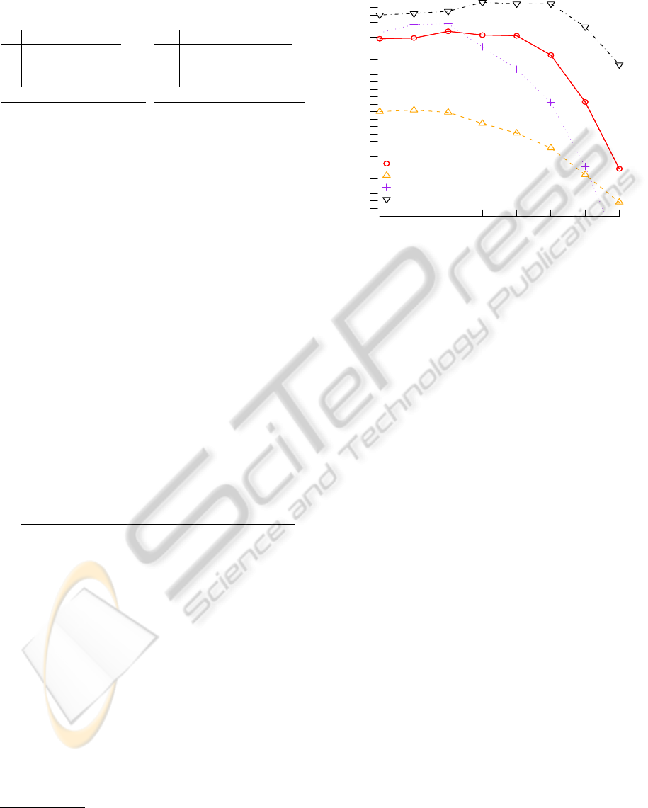
k values
% accuracy
1 5 10 20 30 50 100 200
40 43 46 49 52 55 58 61 64 67
untrained stochasticuntrained stochastic
trained stochastic unsmoothed
trained stochastic smoothed
unit costs
Figure 5: Categorisation performance with unit costs and
some stochastic variants.
The first thing to note is that performance with unit-
costs (▽, max. 67.7%) exceeds performance with the
non-adapted C
D
u
(3) costs (◦, max. 63.8%). Though
not shown, this remains the case with far higher set-
tings of the diagonal factor. Performance after ap-
plying EM
V
to adapt costs (△, max. 53.2%) is
worse than the initial performance (◦, max. 63.8%).
A Leave-One-Out evaluation, in which example-set
items are categorised using the method on the remain-
der of the example-set, gives accuracies of 91% to
99%, indicating EM
V
has made the best-scripts con-
necting the training pairs too probable, over-fitting the
cost table. The vocabulary is sufficiently thinly spread
over the training pairs that its quite easy for the learn-
ing algorithm to fix costs which make almost every-
thing but exactly the training pairs have zero proba-
bility. The performance when smoothing is applied
(+,max. 64.8%), interpolating the adapted costs with
the initial cost, with l = 0.99, is considerably higher
than without smoothing (△), attains a slightly higher
maximum than with unadapted costs (◦), but is still
worse than with unit costs (▽).
The following is a selection from the top 1% of
adapted swap costs.
8.50 ? .
8.93 NNP NN
9.47 VBD VBZ
9.51 NNS NN
9.78 a the
11.03 was is
11.03 ’s is
12.31 The the
12.65 you I
13.60 can do
13.83 many much
13.92 city state
13.93 city country
For the data-set used, these learned preferences are to
some extent intuitive, exchanging punctuation marks,

words differing only by capitalisation, related parts of
speech (VBD vs VVZ etc), verbs and their contrac-
tions and so on. One might expect this discounting of
these swaps relative to others to assist the categorisa-
tion, though the results reported so far indicate that it
did not.
Recall that the cost-table for the stochastic edit
distance is a representation of probabilites, with prob-
abilities represented by their negated base-2 loga-
rithms. A 0 in this case represents the probability
1. Because in a stochastically valid cost table, the
sum over all the represented probabilities must be 1,
a single 0 entry in a cost table implies infinite cost
entries everywhere else. This means that a stochasti-
cally valid cost table cannot have zero costs on the
diagonal, which is the situation of the unit-cost ta-
ble, C
01
. This aspect perhaps mitigates against suc-
cess. The diagonal factor d in the cost initialisation
is designed to make the entries on the diagonal more
probable than other entries, but even with very high
values for d, indicating a high ratio between the diag-
onal and off-diagonal probabilities, the diagonal costs
are not negligible. This means that the unit-cost set-
ting, C
01
, which is clearly ’uniform’ in a sense, is not
directly emulated by the ’uniform’ stochastic initiali-
sations C
D
u
(d). The performance with the unadapted
uniform stochastic initialisation was below the perfor-
mance with unit-costs. Although results in Figure 5
show just the outcomes with C
u
(3), this remained the
case with far larger values of the diagonal factor d.
This invites consideration of outcomes if a final step
is applied in which all the entries on the cost-table’s
diagonal are zeroed. In work on adapting cost-tables
for a stochastic version of string distance used in du-
plicate detection, (Bilenko and Mooney, 2003) used
essentially this same approach. Figure 6 shows out-
comes when the trained and smoothed costs finally
have the diagonal zeroed.
The (▽) series once again shows the outcomes with
unit-costs. In this experiment, with the diagonal
zeroed, this is necessarily also the outcome ob-
tained with any unadapted uniform stochastic ini-
tialisation C
D
u
(d). The other lines in the plot
show the outcomes obtained with costs adapted by
EM
V
, smoothed at varius levels of interpolation (l ∈
{0.99, 0.9, 0.5,0.1}) and with the diagonal zeroed.
Now the unit costs base-line is clearly out-performed,
the best result being 72.5% (k = 20, l = 0.99), as
compared to 67.5% for unit-costs (k = 20). Also bet-
ter results are obtained with the higher levels of the
interpolation factor, indicating greater weight given to
the values obtained by EM
V
and less to the stochastic
initialisation.
k values
% accuracy
1 5 10 20 30 50 100 200
60 62 64 66 68 70 72
lam 0.99lam 0.99
lam 0.9
lam 0.5
lam 0.1
unit costs
Figure 6: Categorisation performance: adapted costs with
smoothing and zeroing.
6 CONCLUSIONS
One can tentatively conclude on the basis of these ex-
periments that the Viterbi EM cost-adaptation can in-
crease the performance of a tree-distance based clas-
sifier, and improve it to above that attained in the unit-
cost setting, though this does require smoothing of de-
rived probabilites and a final step of zeroing the diag-
onal.
Experiments with further data-sets is required.
One type of data of interest would be the digit-
recognition data-set represented by a tree-encoding
of outline looked at by (Bernard et al., 2008). It
would also be interest to look at applications not
to do with categorisation per-se. For example, in
the NLP-related tasks of question-answering and en-
tailment recognition, the aim is assess pairs of sen-
tences for their likelihood to be a question-answer or
hypothesis-conclusion pair. A training set of such
pairs could also serve as potential input to the cost
adaptation algorithm.
Alignments between different pairs of trees can
end up being represented by the same edit-script. A
minimal example is that the script (a, A)(b,B)(c,C)
can serve to connect both the pairs (t1,t2) and
(t1
′
,t2
′
), where:
t1 : (c(a)(b)) t2 : (C(A)(B))
t1
′
: (c(b(a))) t2
′
: (C(B(A)))
Therefore the All-script and Viterbi-script
stochastic edit-distances are only a step towards a
fully fledged generative model of aligned trees. A
fully-fledged model would include further factors
to divide the probability P(a,A) × P(b,B) × P(c,C)

between the tree-pairs. A direction for further work
is the investigation of such a model of aligned trees,
and how it relates to some other recent proposals
concerning adaptive tree measures such as (Takasu et
al., 2007), (Dalvi et al., 2009)
ACKNOWLEDGEMENTS
This research is supported by the Science Foundation
Ireland (Grant 07/CE/I1142) as part of the Centre for
Next Generation Localisation (www.cngl.ie) at Trin-
ity College Dublin.
REFERENCES
Bened´ı, J.-M. and S´anchez, J.-A. (2005). Estimation of
stochastic context-free grammars and their use as lan-
guage models. Computer Speech and Language,
19(3):249–274.
Bernard, M., Boyer, L., Habrard, A., and Sebban, M.
(2008). Learning probabilistic models of tree edit dis-
tance. Pattern Recogn., 41(8):2611–2629.
Bilenko, M. and Mooney, R. J. (2003). Adaptive duplicate
detection using learnable string similarity measures.
In Proceedings of the Ninth ACM SIGKDD Interna-
tional Conference on Knowledge Discovery and Data
Mining (KDD-2003), pages 39–48.
Boyer, L., Habrard, A., and Sebban, M. (2007). Learning
metrics between tree structured data: Application to
image recognition. In Proceedings of the 18th Euro-
pean Conference on Machine Learning (ECML 2007),
pages 54–66.
CCG (2001). corpus of classified questions by Cog-
nitive Computation Group, University of Illinois
l2r.cs.uiuc.edu/∼cogcomp/Data/QA/QC.
Dalvi, N., Bohannon, P., and Sha, F. (2009). Robust web ex-
traction: an approach based on a probabilistic treeedit
model. In SIGMOD 09: Proceedings of the 35th
SIGMOD international conference on Management of
data, pages 335–348, New York, NY, USA. ACM.
Dempster, A., Laird, N., and Rubin, D. (1977). Maximum
likelihood from incomplete data via the em algorithm.
J. Royal Statistical Society, B 39:138.
Dudani, S. (1976). The distance-weighted k-nearest neigh-
bor rule. IEEE Transactions on Systems, Man and Cy-
bernetics, SMC-6:325–327.
Emms, M. (2011). Tree-distance code and datasets reported
on in experiments www.scss.tcd.ie/Martin.Emms/
TreeDist.
Emms, M. and Franco-Penya, H.-H. (2011). On order
equivalences between distance and similarity mea-
sures on sequences and trees. In Proceedings of
ICPRAM 2012 International Conference on Pattern
Recognition Application and Methods.
Judge, J. (2006a). Corpus of syntactically annotated ques-
tions http://www.computing.dcu.ie/jjudge/qtreebank/.
Judge, J. (2006b). Adapting and Developing Linguistic Re-
sources for Question Answering. PhD thesis, Dublin
City University.
Judge, J., Cahill, A., and van Genabith, J. (2006). Ques-
tionbank: creating a corpus of parse-annotated ques-
tions. In ACL 06: Proceedings of the 21st Interna-
tional Conference on Computational Linguistics and
the 44th annual meeting of the ACL, pages 497–504,
Morristown, NJ, USA. Association for Computational
Linguistics.
Kuboyama, T. (2007). Matching and Learning in Trees.
PhD thesis, Graduate School of Engineering, Univer-
sity of Tokyo.
Ristad, E. S. and Yianilos, P. N. (1998). Learning string edit
distance. IEEE Transactions on Pattern Recognition
and Machine Intelligence, 20(5):522–532.
Tai, K.-C. (1979). The tree-to-tree correction problem.
Journal of the ACM (JACM), 26(3):433.
Takasu, A., Fukagawa, D., and Akutsu, T. (2007). Statisti-
cal learning algorithm for tree similarity. In ICDM 07:
Proceedings of the 2007 Seventh IEEE International
Conference on Data Mining, pages 667672, Washing-
ton, DC, USA. IEEE Computer Society.
Wagner, R. A. and Fischer, M. J. (1974). The string-tostring
correction problem. Journal of the Association for
Computing Machinery, 21(1):168–173.
Zhang, K. and Shasha, D.(1989). Simple fast algorithms for
the editing distance between trees and related prob-
lems. SIAM Journal of Computing, 18:1245–1262.
APPENDIX
Proof Concerning Out of Table Costs
Let C
D
be a cost-table associated with a given label
alphabet S , let T be a tree with n symbols 6∈ S , and let
k be a fixed, out-of-table cost for any (x,u), where x ∈
S ∪ {l }, u 6∈ S . Suppose S is a tree whose labels are
in S . Every s ∈ E(S,T) involve n out-of-table events.
SupposeV is the least-cost script, with cost cost
k
(V ).
Now suppose under a higher setting of k
′
for out-of-
table costs, that V
′
6= V is the least-cost script, so
cost
k
′
(V
′
) < cost
k
′
(V ). But recosting according to k
gives cost
k
(V
′
) < cost
k
(V ), which contradicts min-
imality of V under k . So the minimal script is in-
variant to changes of k , and D
v
k
′
(S,T) − D
v
k
(S,T) =
n× (k − k
′
). It follows that neighbour ordering is in-
variant to changes of k .
