
ADAPTIVE SEARCH-BASED HIERARCHICAL MOTION
ESTIMATION USING SPATIAL PRIORS
Michael Santoro, Ghassan Al-Regib, and Yucel Altunbasak
School of Electrical and Computer Engineering, Georgia Institute of Technology, Atlanta, GA, U.S.A.
Keywords:
Block Matching, True Motion Estimation (ME), HBM: Smoothness Constraints, Regularization, Recursive
Search (RS).
Abstract:
Since motion estimation via block matching is an ill-posed problem, it requires the use of smoothness con-
straints to regularize the motion field. The block matching error and smoothness constraints together form an
energy expression to be minimized. Motion vectors (MVs) from a candidate set are used to determine which
MV minimizes the overall energy. These MVs, which may consist of spatial or temporal MVs, determine the
quality of the motion field. Therefore, to ensure a high-quality motion field, we propose a new method to
improve the quality of the MVs. The proposed method uses a novel approach to incorporate prior spatial MVs
into block matching. By incorporating these MVs into block matching, we significantly reduce the size of the
candidate set and improve the quality of the motion field.
1 INTRODUCTION
Accurate motion estimation has become a defining
factor in applications such as video compression,
object tracking, frame-rate conversion, and super-
resolution (de Haan, 2000). To enable real-time ap-
plications, block-matching-based motion estimation
is frequently chosen for its ease of implementation
and low hardware complexity. However, motion es-
timation via block matching is an ill-posed problem,
and block matching alone is not sufficient for gen-
erating motion fields that represent the true motion
of objects. Therefore, it is necessary to introduce
regularization (“smoothness”) constraints in order to
solve the ill-posed nature of block matching. In pre-
vious works (Yin et al., 2006)(Bartels and de Haan,
2010)(Tai et al., 2008)(Huska and Kulla, 2007)(Chen
et al., 1996)(de Haan et al., 1993), smoothness con-
straints were applied following a coarse estimation of
the motion field via block matching. In this paper,
however, we introduce a novel method that incorpo-
rates smoothness constraints into both block matching
and subsequent refinement of the motion field.
Block matching makes use of the translational-
motion model and brightness-constancy assumption
to estimate the motion of blocks between image pairs.
Block matching methods in the literature almost ex-
clusively use the Sum of Absolute Deviations (SAD)
correlation metric, which computes the L1 norm of
pixel differences. However, for brightness variations,
uniform regions, repeating patterns, and complex mo-
tions such as rotation and zooming, block match-
ing has been shown to perform poorly (Kordasiewicz
et al., 2007).
To regularize the ill-posed nature of block match-
ing, i.e., to convert the motion estimation prob-
lem into a convex problem, smoothness constraints
have been introduced (Yin et al., 2006)(Bartels and
de Haan, 2010). Smoothness constraints operate on
the assumption that the motion field generated via
block matching should be locally constant. It has been
shown (Bartels and de Haan, 2010)(de Haan et al.,
1993) that improvements in the quality of the motion
field can be made by forming a candidate set of spa-
tiotemporal MVs around the reference MV, and by
choosing an edge-preserving smoothness constraint
which penalizes deviations among MVs. The spa-
tiotemporal MVs that form the candidate set may in-
clude temporal MVs from previous image pairs in an
image/video sequence, spatial MVs from the current
image pair, and/or spatial MVs from a hierarchy gen-
erated on the current image pair. However, we re-
strict our development in this paper to spatial MVs
and leave temporal MVs for future work.
The remainder of this paper is organized as fol-
lows. In section 2, we combine both block match-
ing and regularization into a Bayesian framework to
develop an expression for minimizing the overall en-
399
Santoro M., Al-Regib G. and Altunbasak Y..
ADAPTIVE SEARCH-BASED HIERARCHICAL MOTION ESTIMATION USING SPATIAL PRIORS.
DOI: 10.5220/0003865003990403
In Proceedings of the International Conference on Computer Vision Theory and Applications (VISAPP-2012), pages 399-403
ISBN: 978-989-8565-04-4
Copyright
c
2012 SCITEPRESS (Science and Technology Publications, Lda.)

ergy. An overview of the HBM framework is dis-
cussed in section 3. In section 4, we discuss our novel
method of using smoothness constraints within the
HBM framework. Experimental results are shown in
section 5, and the conclusions of the paper are pre-
sented in section 6.
2 ENERGY MINIMIZATION
2.1 Bayesian Framework
In this section, we develop a Bayesian framework that
combines the SAD and smoothness constraints to de-
termine which MV from the candidate set minimizes
the overall energy. In order to minimize the energy
expression, we assume that a coarse estimation of the
motion field has been obtained using SAD minimiza-
tion only.
We wish to maximize the probability of choos-
ing a MV given the SAD error between motion-
compensated blocks in the adjacent image and the
spatial MVs of blocks in the current image. The MV
v
i
for the block under consideration in the current im-
age and its spatial MVs v
s
form a set of candidate
MVs, V
k×k
, where k ×k is the size of the neighbor-
hood. Using Bayes’ theorem, we relate the current
MV to the SAD error and spatial MVs as follows:
p(v
i
| d, v
s
) =
p(d | v
i
, v
s
)p(v
i
| v
s
)
p(d | v
s
)
, (1)
where d is the SAD error between the motion-
compensated blocks, v
s
contains the spatial MVs, and
v
i
is one of the MVs from V
k×k
. We now examine
each term on the right-hand side of (1). The first term,
p(d | v
i
, v
s
), can be written as p(d | v
i
) since the error
d only depends on the current MV and not its spa-
tial neighbors. If we assume that the error is additive,
white, Gaussian noise, then p(d | v
i
) can be rewritten
as
p(d | v
i
) =
1
√
2πσ
2
×
exp
(
−
1
2σ
2
∑
x∈B
|
y
k
(x) −y
k−1
(x + v
i
)
|
)
, (2)
where σ
2
is the variance of the pixel differences, x is
the pixel position within a square pixel block B, and
y
k
, y
k−1
represent the current and adjacent images, re-
spectively. From (2), it can be seen that each pixel
within block B of the current image y
k
(x) is subtracted
from the corresponding motion-compensated pixel in
the adjacent image, y
k−1
(x + v
i
).
The second term on the right-hand side of (1),
p(v
i
| v
s
), denotes the conditional probability of MV
v
i
given the spatial MVs, v
s
. This term represents
the prior term in the Bayesian formulation, and un-
der the assumption of having Markovian properties,
can be expressed as a realization of a Gibbs random
field (Konrad and Dubois, 1992). We therefore ex-
press p(v
i
| v
s
) as a Gibbs distribution as follows:
p(v
i
| v
s
) =
1
Z
exp
{
−U(v
i
| v
s
)
}
, (3)
where Z is a normalizing constant and U(v
i
| v
s
) is an
energy function which measures the similarity of MV
v
i
to the spatial MVs, v
s
. We use the energy function
to define the “smoothness” of the MV field. A MV
field is described as smooth if the differences between
the current MV and spatial MVs is small. To charac-
terize the smoothness, we wish to find a robust metric
which penalizes the deviation of MVs. Therefore, we
express the energy function of (3) as
U(v
i
| v
s
) =
∑
j∈v
s
V (v
i
, v
j
), (4)
where V (v
i
, v
j
) is a function which assigns a penalty
to the deviation of v
i
and v
j
.
The term in the denominator of (1) is not a func-
tion of v
i
and can be replaced with a constant. Next,
we combine (2), (3), and (4) to maximize the right-
hand side of (1).
To find the MV ˆv
i
which maximizes the right-hand
side of (1), i.e.,
ˆv
i
= argmax
i
p(d | v
i
, v
s
)p(v
i
| v
s
), (5)
we substitute (2),(3), and (4). Therefore, (5) becomes
ˆv
i
= argmax
i
1
Z
√
2πσ
2
exp
(
−
1
2σ
2
∑
x∈B
|
y
k
(x) −y
k−1
(x + v
i
)
|
−
∑
j∈v
s
V (v
i
, v
j
)
)
.
(6)
An equivalent representation of (6) can be formed by
ignoring the constant terms and minimizing the nega-
tive logarithm, i.e.,
ˆv
i
= argmin
i
(
∑
x∈B
|
y
k
(x) −y
k−1
(x + v
i
)
|
+
∑
j∈v
s
V (v
i
, v
j
)
)
. (7)
To form the equation for the minimizing the overall
energy, we re-write (7) as
E = min
i
SAD(x, x + v
i
) + λ Smoothness(v
i
, v
s
j
)
,
(8)
where E is the overall energy, v
s
j
contains the spa-
tial neighbors of v
i
, and we have introduced Lagrange
multiplier λ to weight the smoothness term.
VISAPP 2012 - International Conference on Computer Vision Theory and Applications
400
2.2 Smoothness Penalty Function
Bartels and Haan (Bartels and de Haan, 2010) eval-
uated the effect of several smoothness constraints on
the quality of the motion field. In our research, we
conducted similar tests for different penalty functions
and neighborhood sizes using the Middlebury test se-
quences (Baker et al., 2011). Similar to (Bartels and
de Haan, 2010), we found the optimal model for the
penalty function as follows:
Smoothness(v
i
, v
s
j
) =
∑
j∈v
s
j
v
i
−v
j
1
, (9)
where
v
i
−v
j
1
denotes the L1 norm between MVs
v
i
and v
j
.
3 HIERARCHICAL BLOCK
MATCHING
3.1 Overview
The basic idea behind Hierarchical Block Matching
(HBM) is to create a pyramid for the pair of images
whose motion we wish to estimate (Bierling, 1988).
Following the creation of a pyramid for each im-
age, the HBM algorithm performs block matching at
each level successively, starting with the lowest res-
olution level (Bierling, 1988). The lowest resolution
level uses large blocks and a modest search size to
determine a rough estimate of the MVs. The MVs
are then passed up to the next higher resolution level
to initialize the search. As the algorithm progresses
to higher resolution levels, the search and block size
may be reduced since an initial estimate was provided
by the previous level.
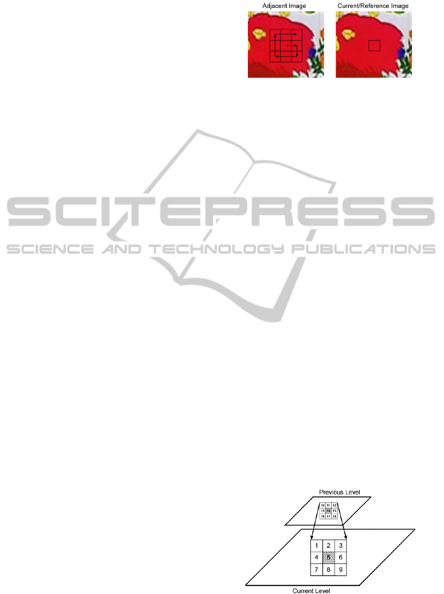
3.2 Search Strategies
Block-matching-based algorithms form a search win-
dow in the adjacent image for the block whose MV
is to be determined, as shown in Fig. 1. Then, a
search for the block that minimizes the SAD error
is performed in raster scan order (top left to bottom
right). To see why raster scan is sub-optimal, con-
sider a block which resides in a uniform region, i.e.,
the majority of the blocks in the search area produce
the same SAD error. In this case, which is shown in
Fig. 1, the block in the top left corner of the search
window will always be selected as the block with the
minimum SAD error.
To improve the likelihood of selecting the best
block in the event that multiple blocks produce the
Figure 1: HBM using spiral search order.
same SAD error, we use a spiral search strategy. Spi-
ral search relies on the observation that the block in
the adjacent image which minimizes the SAD error is
likely to be in the vicinity of the block in the current
image. An example of spiral search is shown in Fig. 1,
where the search direction is indicated by the arrows.
3.3 Candidate Sets
Recall that the MVs in the candidate set are used in
the smoothness constraints and tested in the penalty
function of (9). When utilizing the HBM framework,
the size of the candidate set may be increased after
the MVs for the first (lowest resolution) level of the
hierarchy have been determined. The additional MVs
in the candidate set are taken from the spatial MVs at
the previous level of the hierarchy. If a second-order
neighborhood is used for the smoothness constraints,
the expanded candidate set will consist of 18 spatial
MVs for the desired image pair. The expanded candi-
date set is shown in Fig. 2. As shown in Fig. 2, MV
‘5’ (shaded) is the reference MV for the current level,
and MV ‘14’ (shaded) is the corresponding MV for
the previous level of the hierarchy. To determine the
MV which minimizes the energy, each of the possible
18 MVs may be tested in (8). We refer to this method
as multiple candidate search (MCS), and it is further
described in section 5.2. However, the proposed al-
gorithm introduced in the next section uses a reduced
candidate set of only nine MVs and produces a higher
quality motion field.
Figure 2: Candidate set using two levels of hierarchy.
ADAPTIVE SEARCH-BASED HIERARCHICAL MOTION ESTIMATION USING SPATIAL PRIORS
401

4 SMOOTHNESS CONSTRAINTS
WITHIN HBM
To motivate the methodology in this section, we ex-
amine two possible cases where the block matching
search will fail. For the spiral search strategy in-
troduced in section 3.2, the initial search direction
is ambiguous. Rather than performing the search in
the clockwise direction, the search could also be per-
formed in the counter-clockwise direction. In ad-
dition, the first searched block could be any of the
neighbors.
Figure 3: Examples of images containing multiple matches.
Two cases where multiple matches may exist de-
pending on the search direction are shown in Fig. 3.
The image on the left contains vertical window blinds
which repeat in the horizontal direction. The solid
block in the image represents the block whose MV we
wish to determine, and the blocks with dotted lines
represent possible matches. The image on the right
contains a pattern taken from a textured region. Sim-
ilarly, the solid block represents the block whose MV
we wish to determine, and the blocks with the dotted
lines represent possible matches.
Even in the absence of motion, there are multi-
ple minimums for the blocks in both images. How-
ever, a unique minimum can be found in both im-
ages if a larger block size is used. Fortunately, the
HBM framework is well-suited to handle such cases.
In the HBM framework, the initial level of the hier-
archy contains large blocks which provide an initial
estimate of the motion.
Therefore, we wish to take advantage of the previ-
ous level’s MV to infer the best matching block at the
current level of the hierarchy.
To solve the multiple match problem in Fig. 3,
other works (Bartels and de Haan, 2010)(de Haan
et al., 1993) have introduced new MVs into the can-
didate set by adding normal distributed noise, i.e.,
v
new
=
v
old
+ n | n ∼ N(0, σ
2
)
, (10)
where v
old
is one of the MVs in the original candi-
date set, and v
new
is a new MV introduced into the
candidate set by adding normal distributed noise, n.
However, we do not consider this approach for vari-
ous reasons: 1) It is difficult to determine how many
candidates to include and the value of σ; 2) Since new
candidates are randomly introduced without regard to
the data, it is possible that a false minimum may be
introduced in the candidate set; 3) The computation
time significantly increases as more candidates must
be tested in (8).
4.1 Proposed Method
In the proposed method, we introduce two energy
terms similar to (8). The first term, SAD
min
, repre-
sents the minimum SAD value for the current level of
the hierarchy without regard to any spatial MVs from
the previous level.
The second term, Smoothness
min
, represents the
MV that has the smallest penalty with the previous
level’s MVs for all of the possible positions in the
block matching search range.
We then form the following two expressions:
E
1
= SAD
min
+ Smoothness
1
E
2
= SAD
2
+ Smoothness
min
, (11)
where Smoothness
1
is the penalty (using previous
level’s MVs) for the MV determined by SAD
min
, and
SAD
2
is the SAD value for the block whose MV pro-
duced the Smoothness
min
value.
The decision rule for choosing one of the two pos-
sible MVs is given as follows:
i f (E
2
< E
1
)
choose MV
2
else
choose MV
1
, (12)
where MV
1
is the MV corresponding to E
1
and MV
2
is the MV corresponding to E
2
. The decision rule in
(12) is based on empirical evidence which suggests
that greater preference should be given to the block
which minimizes the SAD error (E
1
) rather than the
block which minimizes the MV penalty, i.e., E
2
.
4.2 Refinement
Following the selection of MV
1
or MV
2
for all of the
blocks in the current image, we may then use the spa-
tial MVs at the current level of the hierarchy to refine
the motion field over multiple iterations using (8). As
will be shown in section 5, the proposed decision rule
in (12) produces a higher quality motion field using
only the spatial MVs for the current level in the re-
finement process; i.e., testing the spatial MVs from
the previous level of the hierarchy in (8) will not fur-
ther improve the quality of the motion field.
VISAPP 2012 - International Conference on Computer Vision Theory and Applications
402

5 RESULTS
In this section, we show that using smoothness con-
straints in HBM improves the quality of the motion
field. All of the results shown in this section were
generated using the Middlebury test sequences with
known ground-truth MVs (Baker et al., 2011).
For our algorithm, we used a three-level hierarchy
for HBM, where the bottom level (highest resolution)
contains the original images interpolated by a factor
of two (to obtain subpixel accurate MVs).
For any given level of the hierarchy, three iter-
ations were performed for each block size, and the
block size was successively reduced down to 2x2
blocks. The execution time for the algorithm was un-
der one second on a 2.8 GHz Intel i7 CPU running a
single thread.
In section 2.1, the Lagrange multiplier λ was in-
troduced. We initialized λ to a small value (twice the
block size) and increased its value as the iterations
progressed.
5.1 Proposed Method vs. MCS
In this section, we compare the proposed method of
introducing smoothness constraints into HBM with
MCS using the endpoint error metric, which is given
as follows:
EE =
q
(u −u
GT
)
2
+ (v −v
GT
)
2
. (13)
In (13), (u, v) is the computed MV and (u
GT
, v
GT
) is
the ground-truth MV. As shown in Table 1, the pro-
posed algorithm results in an improvement for all of
the test sequences. The largest improvement occured
for the “Venus” sequence (0.45dB), and the average
improvement for all sequences was 0.23dB.
6 CONCLUSIONS
As shown in section 5, applying smoothness con-
straints in HBM produced an improvement in the
quality of the motion field without increasing the size
of the candidate set, and possible bad minimums were
not introduced. For the “Grove2”, “Urban3”, and
“Venus” sequences of Table 1, which contain large
motion discontinuities, the proposed algorithm was
shown to significantly outperform the MCS approach.
Even with the improvements produced by smooth-
ness constraints in HBM, there are still cases in which
the motion cannot be accurately estimated (e.g., oc-
clusion, complex motion). In such cases, a validity
metric should be used to characterize the accuracy of
the computed MVs.
Table 1: Improvement of proposed algorithm over MCS.
Image Pair
MCS
Endpoint
Error
Proposed
Endpoint
Error
Improv.
in dB
Grove2
0.353 0.330 0.30dB
Grove3
0.813 0.793 0.11dB
Hydrangea
0.277 0.270 0.11dB
Rubber
0.252 0.245 0.12dB
Urban2
0.579 0.565 0.11dB
Urban3
1.32 1.21 0.38dB
Venus
0.434 0.391 0.45dB
REFERENCES
Baker, S., Scharstein, D., Lewis, J., Roth, S., Black, M.,
and Szeliski, R. (2011). A database and evaluation
methodology for optical flow. International Journal
of Computer Vision, 92:1–31.
Bartels, C. and de Haan, G. (2010). Smoothness constraints
in recursive search motion estimation for picture rate
conversion. IEEE Transactions on Circuits and Sys-
tems for Video Technology, 20(10):1310–1319.
Bierling, M. (1988). Displacement estimation by hierarchi-
cal block matching. In Visual Communications and
Image Processing.
Chen, Y.-K., Lin, Y.-T., and Kung, S. (1996). A fea-
ture tracking algorithm using neighborhood relaxation
with multi-candidate pre-screening. In International
Conference on Image Processing, 1996, volume 2,
pages 513–516.
de Haan, G. (2000). Video processing for multimedia sys-
tems. Eindhoven.
de Haan, G., Biezen, P., Huijgen, H., and Ojo, O. (1993).
True-motion estimation with 3-d recursive search
block matching. IEEE Transactions on Circuits and
Systems for Video Technology, 3(5):368–379, 388.
Huska, J. and Kulla, P. (2007). A new recursive search
with multi stage approach for fast block based true
motion estimation. In 17th International Conference,
Radioelektronika, 2007., pages 1–6.
Konrad, J. and Dubois, E. (1992). Bayesian estimation of
motion vector fields. IEEE Transactions on Pattern
Analysis and Machine Intelligence, 14(9):910–927.
Kordasiewicz, R., Gallant, M., and Shirani, S. (2007).
Affine motion prediction based on translational mo-
tion vectors. IEEE Transactions on Circuits and Sys-
tems for Video Technology, 17(10):1388 –1394.
Tai, S.-C., Chen, Y.-R., Huang, Z.-B., and Wang, C.-C.
(2008). A multi-pass true motion estimation scheme
with motion vector propagation for frame rate up-
conversion applications. Journal of Display Technol-
ogy, 4(2):188–197.
Yin, H. B., Fang, X. Z., Yang, H., Yu, S. Y., and Yang, X. K.
(2006). Motion vector smoothing for true motion esti-
mation. In ICASSP 2006. International Conference on
Acoustics, Speech and Signal Processing, volume 2,
page II.
ADAPTIVE SEARCH-BASED HIERARCHICAL MOTION ESTIMATION USING SPATIAL PRIORS
403
