VISUAL SIMULATION OF MAGNETIC FLUIDS

Tomokazu Ishikawa

, Yonghao Yue

, Kei Iwasaki

, Yoshinori Dobashi

and Tomoyuki Nishita

The University of Tokyo, Tokyo, Japan

Wakayama University, Wakayama, Japan

Hokkaido University, Sapporo, Japan

Keywords:

Magnetic Fluids, SPH (Smoothed Particle Hydrodynamics) Method, Magnet Simulation, Spiking Phe-

nomenon.

Abstract:

In this paper, we focus on simulation of magnetic ﬂuids. Magnetic ﬂuids behave as both ﬂuids and as magnetic

bodies, and these characteristics allow them to generate ‘spike-like’ shapes along a magnetic ﬁeld. Magnetic

ﬂuids are popular materials for use in works of art. Our goal is to simulate such works of art. In the ﬁeld

of electromagnetic hydrodynamics, many methods have also been proposed for simulating such spike shapes

based on numerical ﬂuid analysis. However, those methods are computationally expensive and they typically

require tens of hours just to simulate a single spike. We propose a more efﬁcient method by combining a

procedural approach and the SPH method (smoothed particle hydrodynamics). Our method simulates overall

behaviors of the magnetic ﬂuids using the SPH method and then synthesizes the spike shapes by using the

procedural approach. We demonstrate our method can generate visually plausible results within a reasonable

computational cost.

1 INTRODUCTION

In the ﬁeld of computer graphics, ﬂuid simulation

is one of the most important research topics. Many

methods have therefore been proposed to simulate re-

alistic motion of ﬂuids by introducing physical laws.

Previous methods have attempted to simulate incom-

pressible ﬂuids, such as smoke, water and ﬂames, as

well as compressible ﬂuids such as explosions and

viscous ﬂuids (Stam, 1999) (Fedkiw et al., 2001)

(Goktekin et al., 2004) (Yngve et al., 2000). In this

paper, we focus on visual simulation of magnetic ﬂu-

ids.

A magnetic ﬂuid is a colloidal solution consisting

of micro-particles of ferromagnetic bodies, a surfac-

tant that covers the magnetic micro-particles, and a

solvent that acts as the base (see Fig.1). Therefore,

magnetic ﬂuids behave as both ﬂuids and as magnetic

bodies and can be magnetized and attracted to a mag-

net. Thanks to the controllability of the shapes of the

magnetic ﬂuids by magnetic forces, magnetic ﬂuids

have been widely used for various products such as

electrical and medical equipments. A more interest-

ing application of the magnetic ﬂuids have appeared

for creating new works of art. When a magnet is loca-

Figure 1: Structure material of magnetic ﬂuid.

ted near a magnetic ﬂuid, the magnetic ﬂuid forms

spiky shapes like horns along the direction of the

magnetic ﬁeld generated by the magnet (see Fig. 2).

This is known as the ‘spiking phenomenon’. The

art work using the magnetic ﬂuids utilizes this phe-

nomenon and generates interesting shapes by apply-

ing magnetic forces to the ﬂuids.

Magnetic ﬂuids have been studied extensively in

the ﬁeld of electromagnetic hydrodynamics. The phe-

nomena covered by electromagnetic hydrodynamics

can be further classiﬁed into plasma and magnetic ﬂu-

ids. A plasma is an electromagnetic ﬂuid that gen-

erally has charge (i.e. an electric current ﬂows) but

does not haveanydeﬁned interfaces (or free surfaces).

The dynamics of aurora, prominence, and ﬂares in the

319

Ishikawa T., Yue Y., Iwasaki K., Dobashi Y. and Nishita T..

VISUAL SIMULATION OF MAGNETIC FLUIDS.

DOI: 10.5220/0003867303190327

In Proceedings of the International Conference on Computer Graphics Theory and Applications (GRAPP-2012), pages 319-327

ISBN: 978-989-8565-02-0

 2012 SCITEPRESS (Science and Technology Publications, Lda.)

Figure 2: Spiking phenomenon of magnetic ﬂuid (photo-

graph).

sun can be calculated by simulating a plasma. On

the other hand, a magnetic ﬂuid has usually inter-

faces but does not have any charges. We can ﬁnd a

few researches on the visual simulation of these phe-

nomena in the ﬁeld of computer graphics. However,

to the best of our knowledge, no methods have been

proposed for simulating the magnetic ﬂuids in the

ﬁeld of computer graphics. Although we could use

techniques developed in the ﬁeld of magnetohydro-

dynamics, their computational cost is extremely high

(Yoshikawa et al., 2011). They typically require tens

of hours to simulate a single spike only.

We therefore propose an efﬁcient and visually

plausible method for simulating the spiking phe-

nomenon, aiming at the virtual reproduction of the

art work. Our method combines a procedural ap-

proach and the SPH (smoothed particle hydrodynam-

ics) method. The SPH method is used to compute

overall surfaces of the ﬂuid with a relatively small

number of particles. Then, we generate the spike

shapes procedurally onto the ﬂuid surface. Although

our method is not fully physically-based, it is easy to

implement and we can reproduce spike shapes that are

similar to those observed in the real magnetic ﬂuids.

2 RELATED WORK

Many methods have been proposed to simulate in-

compressible ﬂuids such as smoke and ﬂames (Stam,

1999) (Fedkiw et al., 2001). Goktekin et al. proposed

a simulation method for viscoelastic ﬂuids by incor-

porating an elastic term into the Navier Stokes equa-

tions (Goktekin et al., 2004).

Stam and Fuime introduced the SPH method into

the CG ﬁeld for representing ﬂames and smoke (Stam

and Fiume, 1995). M¨uller et al. proposed a SPH-

based method based to simulate ﬂuids with free sur-

faces (M¨uller et al., 2003). Recently, many methods

using the SPH method have been proposed, e.g., sim-

ulation of viscoelastic ﬂuids (Clavet et al., 2005), in-

teraction of sand and water (Rungjiratananon et al.,

2008), and fast simulation of ice melting (Iwasaki

magnetic

field

magnetic fluid

(a) (b) (c)

Figure 3: Potentiality of shapes of magnetic ﬂuid. (a), (b)

and (c) show the state with minimum potential energy, min-

imum magnetic energy and minimum surface energy, re-

spectively.

et al., 2010). Our method also uses the SPH method

and to simulate the magnetic ﬂuids.

In computer graphics, no methods have been pro-

posed for simulating electromagnetic hydrodynam-

ics. Although a technique for simulating the mag-

netic ﬁeld was proposed by Thomaszewski et al

(Thomaszewski et al., 2008), only the magnetism of

rigid bodies is calculated as an inﬂuence of mag-

netic ﬁelds. Baranoski proposed a visual simulation

method for the aurora by means of simulating the

interaction between electrons and the magnetic ﬁeld

using particles with an electrical charge (Baranoski

et al., 2003) (Baranoski et al., 2005). However, these

methods do not take into account ﬂuid dynamics.

In the ﬁeld of physics, the characteristics of mag-

netic ﬂuids have been studied since 1960. Rosenswig

demonstrated spiking phenomena by using quantita-

tive analysis (Rosensweig, 1987). Sudo et al. have

studied the effects of instability, not only in the spik-

ing phenomenon, but also on the surfaces of mag-

netic ﬂuids (Sudo et al., 1987). Han et al. mod-

eled the formation of a chain-shape between colloidal

particles according to the magnetization of the parti-

cles(Han et al., 2010). Combined with a lattice Boltz-

mann method, they showed that the colloidal parti-

cles would form lines along the magnetic ﬁeld. How-

ever, their method cannot represent the spike shapes.

Yoshikawa et al. combined the MPS (Moving particle

Semi-implicit) method with the FEM (Finite Element

Method) and simulated magnetic ﬂuids. Even when

using 100,000 particles and a mesh with 250,000

tetrahedra, they were able to reproduce only a single

spike (Yoshikawa et al., 2011).

3 SPIKING PHENOMENON

Before explaining our simulation approach, we will

describe the mechanism about the formation of the

spike shape (Rosensweig, 1987). There are three im-

portant potential energies E

, E

mag

and E

that relate

GRAPP 2012 - International Conference on Computer Graphics Theory and Applications

320

to the formation mechanism.

is the potential energy of gravity. If only the

gravity is applied as an external force to the magnetic

ﬂuid, the ﬂuid will form a horizontal surface at a con-

stant height, as shown in Fig. 3 (a), since E

is at

the minimum level under this condition. E

mag

is the

magnetic potential energy. If only the magnetic force

is applied as an external force, the ﬂuid will form a

certain number of spheroids that stand at the bottom

of the vessel, as shown in Fig. 3 (b). E

mag

is at a

minimum level under these conditions. E

is the sur-

face energy. If the surface tension alone is applied as

the external force, the ﬂuid will form into a spherical

shape, as shown in Fig. 3 (c). E

is at the minimum

level under these conditions. The actual shape is the

one that minimizes the summation of these three en-

ergies, resulting in spike-like shapes, as shown in Fig.

Therefore, in order to simulate the spiking phe-

nomena, the three forces need to be taken into ac-

count: the gravity, magnetic forces, and the surface

tension. At the early stages of this research, we tried

to simulate the spiking phenomenon by using the SPH

method only. However, it turned out that we could

not reproduce the spikes unless we used a signiﬁcant

number of particles, resulting in a very long compu-

tation time. Thus, we use the SPH method to simu-

late the overall behavior of the ﬂuids and develop a

new procedural method to generate the spike shapes.

Details of our method is described in the following

sections.

4 OUR SIMULATION METHOD

As we described before, our method combines the

SPH method and a procedural approach. In this sec-

tion, we ﬁrst describe the governing equations of

the magnetic ﬂuid that are solved by using the SPH

method (Section 4.1). Next, we describe the computa-

tion of the magnetic force applied to each particle and

a technique for generating the ﬂuid surface by using

the result of the SPH simulation (Section 4.2). Then,

we describe the procedural method for computing the

spike shape (Section 4.3).

4.1 Governing Equations

The behavior of incompressible ﬂuids is described by

the following equations.

∇·u = 0, (1)

∂u

∂t

= −(u·∇)u−

∇p+ ν∇

u+ F. (2)

Equation (1) is the continuity equation, and Navier-

Stokes equation (Equation (2)) describes the conser-

vation of momentum. u is the velocity vector, t is

time, ρ is the ﬂuid density, p is the pressure and ν is

the kinematic viscosity coefﬁcient. F is the external

force that includes the gravity, the magnetic force, and

the surface tension (Iwasaki et al., 2010).

Our method solves the above equations by using

the SPH method. That is, the magnetic ﬂuids are rep-

resented by a set of particles and the motion of the

ﬂuids is simulated by calculating the motions of the

particles. For this calculation, we use the method de-

veloped by Iwasaki et al (Iwasaki et al., 2010). This

method is signiﬁcantly accelerated by using the GPU

and is capable of simulating water. We extend the

method to the simulation of magnetic ﬂuids. The dif-

ference of magnetic ﬂuids from the non-magnetic ﬂu-

ids is that the magnetic force is induced when mag-

netic ﬁeld exists. The computation of the magnetic

force is described in the next subsection.

4.2 Calculation of Magnetization and

Magnetic Force

Each particle represents a small magnetic ﬂuid ele-

ment, and its motion is calculated by taking into ac-

count the properties of both ﬂuid and magnetic body.

To calculate the magnetic force, our method assumes

the paramagnetism, that is, each particle does not have

any magnetic charges if there is no external magnetic

ﬁeld. However, if a magnetic ﬁeld is applied, each

particle becomes magnetized in the direction along

the applied magnetic ﬁeld. In this paper, we assume

that the magnetic ﬁeld is induced by a bar magnet

placed near the ﬂuid. In order to handle a magnet with

an arbitrary shape, we can use the method developed

by Thomaszewski et al (Thomaszewski et al., 2008).

The magnetic ﬁeld is calculated by approximating

the bar magnet as a magnetic dipole. We assume that

the north and south poles of the magnetic bar have an

equal magnitude of magnetic charge but the signs are

different (positive or negative). When computing the

magnetic force working on each particle, it is not suf-

ﬁcient to calculate only the force induced directly by

the magnetic bar. This is due to the paramagnetism.

When each particle is placed in the magnetic ﬁeld of

the magnetic bar,the particle is magnetized and works

as if it were a small spherical magnet. Therefore, our

method ﬁrst computes the magnetic ﬁeld at equilib-

rium state, taking into account the magnetization of

the particles. After that, the magnetic force for each

particle is calculated. The details are described in the

following.

The magnetic moment m due to a magnetic dipole

VISUAL SIMULATION OF MAGNETIC FLUIDS

321

㻿㻺

bar magnet

SPH particle

㻺

㻿

㻿㻺

(a) (b)

distance between

the poles

position

vector

magnetic

vector

H(r

)

magnetic field lines

due to magnetized particle

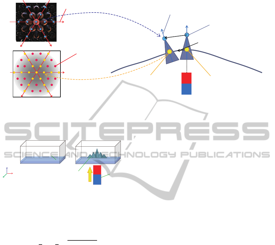
Figure 4: Calculation of the magnetization and the magnetic force. (a) First, we calculate the magnetic ﬁeld vector at each

SPH particle induced by a magnetic dipole. (b) Next, we calculate the inﬂuence of other particles from the magnetized

particles.

Figure 5: Photograph of a real magnetic ﬂuid surface.

Figure 6: The surface computed using Equation (13).

is deﬁned by the following equation:

m = q

d, (3)

where q

is the magnitude of the magnetic charge and

d is a vector connecting from the south to north poles.

We call the magnetic vector induced by the magnetic

bar as a background magnetic vector. Let us assume

that the origin is at the midpoint between the north

and the south poles. Then, the background magnetic

vector H

dipole

(r) at position r is expressed by the fol-

lowing equation.

dipole

(r) = −

4πµ

∇

m·r

, (4)

where µ is the permeability of the magnetic ﬂuid and

r =



. Each particle is magnetized due to the back-

ground magnetic vector ﬁeld and induces an addi-

tional magnetic vector ﬁeld. Thus, in order to obtain

the ﬁnal magnetic vector H(r

) at particle j, the mag-

netic interactions between particles have to be com-

puted by solving the following equation,

H(r

) = H

dipole

) −

4πµ

∑

i=1

i6= j

∇

χH(r

) ·r

, (5)

where V is the volume of a particle and we assume

that the volume of all particles are equal, r

is the po-

sition of particle i, N is the total number of particles, χ

is the magnetic susceptibility. r

= r

− r

, and r

= |

− r

|. The magnetic susceptibility changes due to

the external magnetic ﬁeld. It is known that the mag-

netization of the magnetic ﬂuids is saturated when the

magnitude of an external magnetic ﬁeld is larger. We

calculate the magnetization in all particles based on

the actual relationship between the magnetization and

an external magnetic ﬁeld in (Yoshikawa et al., 2011).

The gradient part of the second term in Equation (5)

is calculated by the following equation,

∇

χH(r

) ·r

= ∇(χH(r

)) ·

+ χH(r

) ·∇(

(6)

We use the kernel function to calculate the partial dif-

ferential of H (r

), that is,

∇(χH(r

)) =

∑

j=1

j6=i

χH(r

)∇w(r

), (7)

where w(r

) is the kernel function. We use the fol-

lowing kernel function frequently refered in the SPH

method (M¨uller et al., 2003),

w(r) =



315

64πh

−r

)

0 ≤ r ≤h

0 h < r,

(8)

where h is the effective radius of each particle. We

calculate Equation (5) taking into account the inﬂu-

ences from all the particles. We use the Gauss-Seidel

method to solve Equation (5).

GRAPP 2012 - International Conference on Computer Graphics Theory and Applications

322

Next, the magnetic force F

mag

) is calculated by

using the following equation (Rosensweig, 1987),

mag

) = −∇φ

), (9)

where,

µ | H(r

) |

. (10)

∇φ

in Equation (9) is calculated by using the kernel

function represented by Equation (8), that is,

∇φ

∑

∇w(r

). (11)

4.3 Computing Spike Shapes

The formation of the small spike shapes on the

magnetic ﬂuid surface can be explained by the bal-

ance among the forces of the surface tension, grav-

ity and the stress due to magnetization (Rosensweig,

1987)DAs we described before, our method synthe-

sizes the spike shapes by employing the procedural

approach. The basic idea is as follows. We prepare a

procedural height ﬁeld representing the spike shapes

generated on a ﬂat surface. Next, during the simula-

tion, the height ﬁeld is mapped onto the curved sur-

face calculated by using the SPH particles. When the

ﬂuid surface is ﬂat and a magnetic ﬁeld is perpendic-

ular to the ﬂat surface, the spike shapes can be rep-

resented as a height ﬁeld z(x, y) expressed by the fol-

lowing equation (see 7 for derivation).

z(x, y) =

∑

(sink

x+C

cosk

x)(sink

y+C

cosk

y),

(12)

where C

(i = 0, 1, 2), k

and k

are parameters con-

trolling the spike shapes. There is a constraint on k

and k

: these need to be integers that satisfy k

+ k

is the same for possible combinations of k

and k

. Σ

means the sum of the possible combinations. For the

real magnetic ﬂuids, a regular hexagonal pattern is of-

ten observed (see Fig. 5). Therefore, we choose the

constants in Equation (12) so that such a pattern can

be reproduced:

z(x, y) = C

(cos

(

√

3x+ y) + cos

(

√

3x−y) + cosky).

(13)

The above equation is used for the procedural height

ﬁeld representing the spike shapes on a ﬂat surface.

We set k to 50. Fig. 6 shows an example of the spike

shapes synthesized by using Equation (13). Com-

pared to Fig. 5, we can see that the synthesized shape

is very similar to the real spike shapes. The size of

the spike is controlled by adjusting C

. We simply as-

sume that C

is proportional to the magnitude of the

magnetic ﬁeld.

= β | H(x) |, (14)

where, β is the proportional coefﬁcient, | H(x) | is the

magnitude of the magnetic ﬁeld at position x.

In the real world, the following three structural

features are observed: 1) positions of the spikes are

symmetric as shown in Fig. 5, 2) distances between

neighboring spikes become shorter when the mag-

netic force becomes stronger, and 3) the spikes are

formed along the direction of the magnetic ﬁeld lines.

We develop a mapping method so that these three fea-

tures are reproduced.

First, we set the intersection between the extended

line connecting a magnetic dipole and the ﬂuid sur-

face to the origin of the texture coordinate deﬁned by

xy in Equation (13). This is because the magnetic ﬁeld

created from one magnet becomes symmetrical ﬁeld

with respect to a point centering on magnet. We trace

six directions from the origin of the texture coordi-

nates and calculate the mapping coordinates of the

vertices of the spike because the height ﬁeld repro-

duced by Equation (13) has three axes of symmetry

(see Fig. 7 (a)). Let x

be the position of the top of

the spike just above the magnet. For each direction of

six tangent vectors align to the three axes, the posi-

tion of n-th spike x

from the origin is calculated by

the following equation,

= x

n−1

+ l(H(x

))d

n−1

, (15)

where l is a function representing the distance be-

tween the tops of n −1-th and n-th spikes and it is

determined by H(x

). d

n−1

is the tangent vector on

the ﬂuid surface at the mapping coordinate s

n−1

. Ex-

perimentally, we used l =

|H(x

, where α = 0.15.

To represent the characteristics that the spikes

grow along the direction of the magnetic ﬁeld lines,

we calculate the magnetic ﬁeld vector at x

, and we

calculate the intersection between the ﬂuid surface

and the magnetic ﬁeld vector. The intersection point

is the mapping coordinate s

. By repeatedly apply-

ing this operation to a mapping area, we calculate the

mapping coordinates.

The positions of the tops of the spikes between

two adjacent symmetry axes (red points in Fig. 7 (c))

are calculated by interpolating the positions of two n-

th spikes (yellow points in Fig. 7 (c)).

The mapping area is determined by using the par-

ticles whose magnitudes of the magnetizations are

greater than a threshold. The magnitude of magne-

tization is calculated by the balanced equation (Equa-

tion (26)) for simple spike shapes in equilibrium (see

7). We use the minimum value of the magnetization

as the threshold. M

is calculated by the following

equation,

VISUAL SIMULATION OF MAGNETIC FLUIDS

323

magnetic field vector

tangent vector

mapping coordinate

( )

H x

spike coordinate

( )

1 1 1

= +

s x H x

fluid surface

㻺

㻿

mapping coordinate

( )

0 0 0 1

l+ =x H x d x

texture

coordinate

simulation

coordinate

interpolation point

axis of symmetry

(a)

(b)(c)

Figure 7: (a) Spike texture coordinates are used as the height ﬁeld. (b) To calculate the coordinates of the spike vertices, we

trace along the ﬂuid surface. (c) The coordinates other than an axis of symmetry are calculated by interpolation.

㹌

㹑

SPH particles

representing

magnetic fluid

change of the fluid

surface influenced by

the magnetic field

(a) (b)

magnet

Figure 8: The simulation space of our method. (a) The mag-

netic ﬂuids, which are represented by a set of SPH particles,

are stored in a cubic container. (b) The magnet is located

underneath the container. Then the motions of the magnet

ﬂuids are simulated by moving the magnet.

(1+

)

(ρ

−ρ

)gκ, (16)

where ρ

and ρ

are the density of the magnetic ﬂuid

and air, respectively. κ is the magnitude of the surface

tension.

5 RENDERING

The surfaces of the magnetic ﬂuids are extracted by

using the method proposed by Yu et al. (Yu and Turk,

2010). Since the magnetic ﬂuids are colloid ﬂuids, the

transmitted light in the magnetic ﬂuids is scattered.

However, since the colors of the magnetic ﬂuids are

black or brown in general, the albedo of magnetic ﬂu-

ids is very small. Thus, the light scattering effects in-

side the magnetic ﬂuids are negligible. Therefore, our

method ignores the light scattering inside the mag-

netic ﬂuids. We used POV-Ray to render the surfaces.

6 RESULTS

For the simulation of our method, we used CUDA

for the SPH method and the calculation of the mag-

netic force at each SPH particle. The number of par-

ticles used in the simulation shown in Figs. 9 and

10 is 40,960. The average computation time of the

simulation for a single time-step is 6 milliseconds

on a PC with an Intel(R) Core(TM)2 Duo 3.33GHz

CPU, 3.25GB RAM and an NVIDIA GeForce GTX

480 GPU. The parameters used in the simulation are

shown in Table 1. The average computation time of

the surface construction for a frame is 2 minutes on

the same PC. The initial ﬂuid surface is shown in Fig.

8 (a). The ﬂuid is contained in a box, which is not

shown. Fig. 8 (b) shows how the shape of the ﬂuid

surface changes when a magnet approaches the bot-

tom of the box. Fig. 9 shows an animation sequence

of the magnetic ﬂuid when we move the magnet in

the vertical direction. As shown in Fig. 9, the spikes

grow and increase when the magnet moves closer to

the magnetic ﬂuids. Fig. 10 shows an animation se-

quence of the magnetic ﬂuid when we eliminate the

magnet ﬁeld. The surface becomes ﬂat as we decrease

the magnitude of the magnetic ﬁeld. These results

demonstrate that our method can simulate the para-

magnetic property of magnetic ﬂuids. Fig.9 shows

an animation of magnetic ﬂuids with the movement

of a magnet. As shown in Fig.9, the spikes grow

and increase when we move the magnet closer to the

magnetic ﬂuids. These results demonstrate that our

method can simulate the paramagnetic property of

magnetic ﬂuids. Fig. 11 shows an example where we

use two magnets. Compared to the case when using

only a single magnet, the directions of the spikes get

GRAPP 2012 - International Conference on Computer Graphics Theory and Applications

324

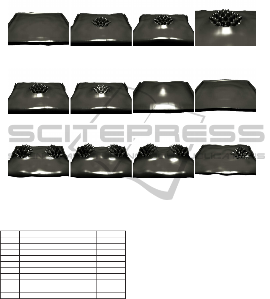
(a) t = 1.6 sec. (b) t = 3.2 sec. (c) t = 4.8 sec.

(d) Enlarged view of (c).

Figure 9: Formation of spikes in the magnetic ﬂuids. Spike shapes grow as the magnet approaches the bottom of the magnetic

ﬂuids.

(a) t = 5.2 sec. (b) t = 6.8 sec. (c) t = 8.4 sec. (d) t = 10.0 sec.

Figure 10: Magnet ﬂuids act as ﬂuids when the magnetic ﬁeld is reduced.

(a) t = 5.2 sec. (b) t = 6.8 sec. (c) t = 8.4 sec.

(d) Using only a single

magnet.

Figure 11: (a) to (c) show the results of the magnet ﬂuids and the spikes by setting two magnets under the magnetic ﬂuids. (d)

shows the simulation result of the spikes using a single magnet for comparison. Compared with (d), the spikes closer to the

other magnet get mush distorted in (a) to (c), the spikes which are closer to the other magnet get much distorted.

Table 1: Parameter setting of magnetic ﬂuid simulation.

param. meaning value

dt time step 0.00075

ν kinematic viscosity coefﬁcient 0.12

m particle mass 0.016

R particle radius 0.5

h effective radius 1.3

g gravitational acceleration 9.8

k coefﬁcient of surface tension 7.5

magnitude of the magnetic charge 5.0

µ permeability of the magnetic ﬂuid 4 π × 10

−7

χ magnetic susceptibility 0.01

changed according to the change in the magnetic ﬁeld

due to the other magnet.

7 CONCLUSIONS AND FUTURE

WORK

We have proposed a visual simulation method for

magnetic ﬂuids whose shapes change according to

the magnetic ﬁeld. We compute the spike shapes us-

ing a procedural approach, and map the shapes onto

the ﬂuid surface. Our method demonstrates that the

magnitude of the magnet ﬁeld inﬂuences the shapes

of the magnet ﬂuids and the magnet ﬂuids act as ﬂu-

ids when the magnet ﬁeld is eliminated. There are

three limitations for our method. First, the conserva-

tion of the ﬂuid volume is not considered when map-

ping the spike shapes onto the ﬂuid surface. Second,

our method cannot handle the fusion of more than one

spike shapes, while we can observe such a fusion in

real magnetic ﬂuids. Third, our method does not sim-

ulate the ﬂows of spikes along the velocity and vortic-

ity of the magnetic ﬂuid, since the function used for

representing the spike shapes is not changed by the

ﬂuid behavior.

In future work, we would like to calculate the

spike pattern other than regular hexagonal pattern dy-

namically using Equation (12) and represent the other

spike shape arrangement. Moreover, to apply our

method to works of art, we would like to control the

magnetic ﬁeld by using electric current ﬂows.

VISUAL SIMULATION OF MAGNETIC FLUIDS

325

REFERENCES

Baranoski, G., Rokne, J., Shirley, P., Trondsen, T., and Bas-

tos, R. (2003). Simulation the aurora. Visualization

and Computer Animation, 14(1):43–59.

Baranoski, G., Wan, J., Rokne, J., and Bell, I. (2005). Sim-

ulating the dynamics of auroral phenomena. ACM

Transactions on Graphics (TOG), 24(1):37–59.

Clavet, S., Beaudoin, P., and Poulin, P. (2005). Particle-

based viscoelastic ﬂuid simulation. In Proceedings of

the 2005 ACM SIGGRAPH/Eurographics symposium

on Computer animation, pages 219–228. ACM, ACM.

Cowley, M. D. and Rosensweig, R. E. (1967). The interfa-

cial stability of a ferromagnetic ﬂuid. Journal of Fluid

Mechanics, 30(4):671–688.

Fedkiw, R., Stam, J., and Jensen, H. W. (2001). Visual sim-

ulation of smoke. In Proceedings of SIGGRAPH 2001,

Computer Graphics Proceedings, Annual Conference

Series, pages 15–22. ACM, ACM Press / ACM SIG-

GRAPH.

Goktekin, T. G., Bargteil, A. W., and OfBrien, J. F. (2004).

A method for animating viscoelastic ﬂuids. In Pro-

ceedings of SIGGRAPH 2004, Computer Graphics

Proceedings, Annual Conference Series, pages 463–

468. ACM, ACM Press / ACM SIGGRAPH.

Han, K., Feng, Y. T., and Owen, D. R. J. (2010). Three-

dimensional modelling and simulation of magnetorhe-

ological ﬂuids. International Journal for Numerical

Methods in Engineering, 84(11):1273–1302.

Iwasaki, K., Uchida, H., Dobashi, Y., and Nishita, T. (2010).

Fast particle-based visual simulation of ice melting.

Computer Graphics Forum (Paciﬁc Graphics 2010),

29(7):2215–2223.

M¨uller, M., Charypar, D., and Gross, M. (2003).

Particle-based ﬂuid simulation for interactive appli-

cations. In Proceedings of the 2003 ACM SIG-

GRAPH/Eurographics symposium on Computer ani-

mation, pages 154–159. ACM, ACM.

Rosensweig, R. (1987). Magnetic ﬂuids. Annual Review of

Fluid Mechanics, 19:437–461.

Rungjiratananon, W., Szego, Z., Kanamori, Y., and Nishita,

T. (2008). Real-time animation of sand-water inter-

action. Computer Graphics Forum (Paciﬁc Graphics

2008), 27(7):1887–1893.

Stam, J. (1999). Stable ﬂuids. In Proceedings of SIG-

GRAPH 1999, Computer Graphics Proceedings, An-

nual Conference Series, pages 121–128. ACM, ACM

Press / ACM SIGGRAPH.

Stam, J. and Fiume, E. (1995). Depicting ﬁre and other

gaseous phenomena using diffusion processes. In

Proceedings of SIGGRAPH 1995, Computer Graphics

Proceedings, Annual Conference Series, pages 129–

136. ACM, ACM Press / ACM SIGGRAPH.

Sudo, S., Hashimoto, H., Ikeda, A., and Katagiri, K. (1987).

Some studies of magnetic liquid sloshing. Journal of

Magnetism and Magnetic Materials, 65(2):219–222.

Thomaszewski, B., Gumann, A., Pabst, S., and Strasser, W.

(2008). Magnets in motion. In Proceedings of SIG-

GRAPH Asia 2008, Computer Graphics Proceedings,

Annual Conference Series, pages 162:1–162:9. ACM,

ACM Press / ACM SIGGRAPH Asia.

Yngve, G. D., O’Brien, J. F., and Hodgins, J. K. (2000).

Animating explosions. In Proceedings of SIGGRAPH

2000, Computer Graphics Proceedings, Annual Con-

ference Series, pages 29–36. ACM, ACM Press /

ACM SIGGRAPH.

Yoshikawa, G., Hirata, K., Miyasaka, F., and Okaue, Y.

(2011). Numerical analysis of transitional behavior

of ferroﬂuid employing mps method and fem. Mag-

netics, IEEE Transactions on, 47(5):1370–1373.

Yu, J. and Turk, G. (2010). Reconstructing surfaces of

particle-based ﬂuids using anisotropic kernels. In Pro-

ceedings of the 2010 ACM SIGGRAPH/Eurographics

Symposium on Computer Animation, pages 217–225.

ACM, Eurographics Association.

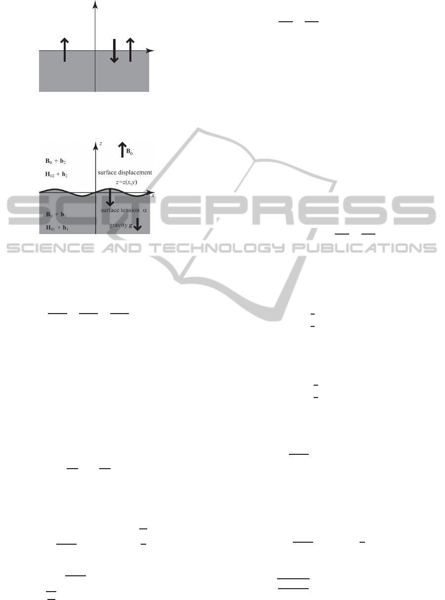
APPENDIX A

Surface Deformation of Magnetic Fluid. In this

appendix, we consider the case where the liquid sur-

face is initially horizontal (the surface is equal to

the xy-plane as shown in Fig. 12) (Cowley and

Rosensweig, 1967). We apply a vertical magnetic

ﬁeld (in z direction) and calculate how the liquid sur-

face changes according to the magnetic ﬁeld. We

show that we can obtain Equation (12) for describing

the surface displacement according to the magnetic

ﬁeld. The variables of the density and magnetic ﬁeld

are deﬁned as shown in Fig 12. When the liquid sur-

face is slightly deformed (Fig. 13), the variation of the

magnetic ﬂux density inside the magnetic ﬂuid, b

B − B

, and the variation of the magnetic ﬁeld, h

H − H

have the following relationship:

= (µh

, µh

, ˆµh

), (17)

where the magnetic ﬂux density and the magnetic

ﬁeld are parallel. µ is the permeability, ˆµ is the dif-

ferential permeability, h

, h

show the x, y and

z components of h

, since the magnetic ﬂux density

and the magnetic ﬁeld are parallel. By letting the

magnetic potential inside the magnetic ﬂuid be φ

the

magnetic ﬁeld h

in case of no electric current can be

expressed as:

= ∇φ

. (18)

If the electric current is ﬂowing, the magnetic ﬁeld

due to electric currents must be considered and the

potential term becomes complicate. By using the fol-

lowing equation,

H = ∇·B, (19)

the divergence of the variation of the magnetic ﬂux

density can be rewritten as:

∇·b

= µ



∂

∂x

∂

∂y



+ ˆµ

∂

∂z

. (20)

GRAPP 2012 - International Conference on Computer Graphics Theory and Applications

326

Magnetic fluid

Air

density

magnetic field H gravity g

magnetic field H magnetic field M

01 01

(> )

Figure 12: Horizontal interfacial boundary and vertical

magnetic ﬁeld. Each character equation of the ﬂuid set as in

the ﬁgure.

Figure 13: Deformation of the interfacial boundary by ap-

plied vertical magnetic ﬁeld.

On the other hand, the magnetic ﬁeld potential φ

above the magnetic ﬂuid satisﬁes the following equa-

tion:



∂

∂x

∂

∂y

∂

∂z



= 0. (21)

Moreover, φ

= 0 (z → − ∞) and φ

= 0 (z →

∞) can be used as boundary conditions because each

magnetic ﬁeld is not affected by the deformation of

the interfacial boundary at z ± ∞. Due to the condi-

tion that the tangential component of magnetic ﬁeld

H is equal on both sides of the liquid surface, and the

surface normal component of magnetic ﬂux density B

has the same value on both sides of the interface, the

following equation is satisﬁed on the deformed liquid

surface.



−φ

= M

z(x, y)

ˆµ

∂φ

∂z

−µ

∂φ

∂z

= 0,

(22)

where, M

= |M

|, z(x, y) is the height ﬁeld of the

deformed liquid surface. Then, the following equa-

tions satisfy Equation (20), (21) and (22) and the

boundary condition.

1+ γ

z(x, y)exp

ˆµ

, (23)

γM

1+ γ

z(x, y)exp(−kz), (24)

where, γ =

ˆµµ

and z(x, y) must satisfy the following

equation:



∂

∂x

∂

∂y

+ k



z(x, y) = 0, (25)

The general solution of this equation is the one

shown in Equation (12).

APPENDIX B

Equilibrium of Force inside Spike Shape. In this

appendix, we explain that the minimum value of the

magnetization is represented as Equation (16) when

the magnetic ﬂuid forms a spike shape. Considering

the balance between the surface tension and the dif-

ference in the stress on both sides of the liquid sur-

face, the equilibrium equation of forces at the liquid

surface can be represented by the following equation

when the spike is formed.

)

−(T

)

−α



∂

∂x

∂

∂y



z = 0, (26)

where T

is the normal stress in z direction and n

the normal vector of z-axis. In the air and the mag-

netic ﬂuid, T

can be written as follows, considering

the magnetic pressure.

)

= −p

+ H

+ B

)

= −p

+ H

+ B

(27)

Substituting the following equation of pressure

distribution in Equation (26),

= −ρ

gz+

−H

)

= −ρ

gz+

−H

(28)

the following equation can be derived considering

Equation (22) and (25),



(ρ

−ρ

)g−

1+ γ

kµ

+ αk



z(x, y) = const.

(29)

Because z is not zero when the spike is deformed,

Equation (29) holds only when the constant on the

right side and the term in parentheses on the left side

are zero.That is,

1+ γ

(ρ

−ρ

)

+ αk

. (30)

If the magnetization of magnetic ﬂuid is less than

Equation (30), the liquid surface does not change.

When k =

(ρ

−ρ

, the right hand side of equation

is minimum. The minimum value is shown in Equa-

tion (16).

VISUAL SIMULATION OF MAGNETIC FLUIDS

327