
SKETCHING FLUID FLOWS
Combining Sketch-based Techniques and Gradient Vector Flow
for Lattice-Boltzmann Initialization
Sicilia Ferreira Judice and Gilson Antonio Giraldi
National Laboratory for Scientific Computing, Petropolis, RJ, Brazil
Keywords:
Fluid Simulation, Lattice-Boltzmann Method, Gradient Vector Flow, Sketching Modeling.
Abstract:
This work proposes an intuitive fluid flow initialization for computer graphics applications. A combination of
sketching techniques and Gradient Vector Flow is proposed to obtain a smooth initialization for the simulation
using a Lattice Boltzmann Method (LBM). The LBM is based on the fundamental idea of constructing simpli-
fied kinetic models, which incorporates the essential physics of microscopic processes so that the macroscopic
averaged properties satisfy macroscopic equations. The application of sketching techniques is proposed in
order to enable the user to draw freely the initial state of the fluid flow using an intuitive interface. Moreover,
it will be possible for the user to define multiply connected domains with suitable boundary conditions.
1 INTRODUCTION
In the last decades, techniques for fluid simulation
have been widely studied for computer graphics ap-
plications. The motivation for such interest relies in
the potential applications of these methods and in the
complexity and beauty of the natural phenomena that
are involved. In particular, techniques in the field
of computational fluid dynamics (CFD) have been
applied for fluid animation in applications such as
virtual surgery simulators (M
¨
uller et al., 2004b), vi-
sual effects (Witting, 1999), and games (M
¨
uller et al.,
2004a).
The traditional fluid animation methods in com-
puter graphics rely on a top-down viewpoint that
uses 2D/3D mesh-based approaches motivated by the
methods of finite element (FE) and finite difference
(FD) in conjunction with Navier-Stokes equations for
fluids (Foster and Metaxas, 1997; Stam, 2003). Al-
ternatively, lattice methods comprised of the Lattice
Gas Cellular Automata (LGCA) and Lattice Boltz-
mann (LBM) can be used. The basic idea behind these
methods is that the macroscopic dynamics of a fluid
are the result of the collective behavior of many mi-
croscopic particles. The LGCA follows this idea, but
it simplifies the dynamics through simple and local
rules for particle interaction and displacements.
On the other hand, the LBM constructs a simpli-
fied kinetic model, a simplification of the Boltzmann
equation, which incorporates the essential micro-
scopic physics so that the macroscopic averaged prop-
erties obey the desired equations (Chen and Doolen,
1998). The LBM have provided significant successes
in modeling fluid flows and associated transport phe-
nomena. The methods simulate transport by tracing
the evolution of a single particle distribution through
synchronous updates on a discrete grid. Before starts
the simulation, it is necessary to define the initial con-
ditions, which can be an initial velocity field, pressure
field or an initial distribution of particles.
The proposal of this work is to provide an intu-
itive fluid flow initialization for the LBM method. To
implement this task, the LBM technique is combined
with methods of sketch-based modeling (Cook and
Agah, 2009). In this way, the user will be able to
define an initial state for the fluid flow through free-
hand drawing. Moreover, it will be possible to set up
holes within the fluid domain in order to get a multi-
ply connected region.
A drawing canvas, which in the actual implemen-
tation is aligned with the computer screen, is provided
to the user. So, the user draws sketch paths inside
the fluid domain using the mouse. Each path defines
a streamline of the fluid and the corresponding tan-
gent field is used to compute the fluid velocity over
the path. Then, this first velocity field is used as input
to the Gradient Vector Flow (GVF) (Xu and Prince,
1997). The field obtained by solving the GVF equa-
tions is a smooth version of the original one that tends
to be extended very far from the user defined paths.
328
Ferreira Judice S. and Antonio Giraldi G..
SKETCHING FLUID FLOWS - Combining Sketch-based Techniques and Gradient Vector Flow for Lattice-Boltzmann Initialization.
DOI: 10.5220/0003868403280337
In Proceedings of the International Conference on Computer Graphics Theory and Applications (GRAPP-2012), pages 328-337
ISBN: 978-989-8565-02-0
Copyright
c
2012 SCITEPRESS (Science and Technology Publications, Lda.)

Thus, the smoothed velocity field is used as an ini-
tial condition for the LBM method. The main con-
tribution of our work is the combination of sketching
techniques and Gradient Vector Flow for LBM initial-
ization.
The article is organized as follows. Section 2 re-
views related works. The section 3 describes the Lat-
tice Boltzmann technique. In section 4 the method-
ology of the Gradient Vector Flow is explained. Sec-
tion 5 explains the sketch-based modeling. In section
6 we describe the proposed technique. The results and
advantages of the proposed framework are shown in
section 7. Finally, section 8 gives the conclusions and
final comments.
2 RELATED WORKS
The LBM method is based on the fundamental idea
of constructing simplified kinetic models that incor-
porate the essential physics of microscopic processes
so that the macroscopic averaged properties satisfy
macroscopic equations. The LBM is especially useful
for modeling complicated boundary conditions and
multiphase interfaces (Chen and Doolen, 1998). Ex-
tensions of this method are described, including sim-
ulations of fluid turbulence, suspension flows, and re-
action diffusion systems (Wei et al., 2004).
Lattice models have a number of advantages
over more traditional numerical methods, particularly
when fluid mixing and phase transitions occur (Roth-
man and Zaleski, 1994). Simulation is always per-
formed on a regular grid, and can be efficiently im-
plemented on a massively parallel computer. Solid
boundaries and multiple fluids can be introduced in a
straightforward manner and the simulation is done ef-
ficiently, regardless of the complexity of the boundary
or interface (Buick et al., 1998). In the case of Lattice-
Gas Cellular Automata (LGCA), there are no numer-
ical stability issues because its evolution follows inte-
ger arithmetic. For LBM, numerical accuracy and sta-
bility depend on the Mach number (max-speed/speed
of sound). The computational cost of the LGCAs is
lower than that for LBM-based methods. However,
system parametrization (e.g., viscosity) is difficult to
do in LGCA models, and the obtained dynamics is
less realistic than for LBM.
To provide an intuitive modeling of the initial
configuration of the fluid, sketching techniques
can be applied. The first sketch-based modeling
system was Sketchpad launched in 1963 by Ivan
Sutherland (Sutherland, 1964), who wrote ”The
Sketchpad system makes it possible for a man and a
computer to converse rapidly through the medium of
line drawings”. An early approach was to use draw-
ing input as symbolic instructions (Zeleznik et al.,
2006). This method allows a designer access to the
multitude of commands in a modeling interface, and
was well suited to the limitations of early hardware.
As technology has progressed, the evolution of these
approach leads to a system that can interpret a user’s
drawing directly (Varley et al., 2004), a system that
can use shading and tone to give a 2D drawing the
appearance of 3D volume (Williams, 1990), and
a system that can approach 3D modeling from the
perspective of sculpture in which virtual tools are
used to build up a model like clay, or cut it down with
tools like a sculptor (Bærentzen and Christensen,
2002).
The sketch-based modeling systems
SKETCH (Zeleznik et al., 2006) and Teddy (Igarashi
et al., 2007) are examples of how sketches or drawn
gestures can provide a powerful interface for fast ge-
ometric modeling. However, the notion of sketching
a motion is less well-defined than that of sketching an
object. Walking motions can be created by drawing
a desired path on the ground plane for the character
to follow, for example. In (Thorne et al., 2004), the
authors present a system for sketching the motion
of a character. Recently, the work of (Schroeder
et al., 2010) proposed a sketch-based system for
creating illustrative visualizations of 2D vector fields.
The work proposed by (Zhu et al., 2011) presents
a sketching system that incorporates a background
fluid simulation for illustrating dynamic fluid sys-
tems. It combines sketching, simulation, and control
techniques in one user interface and can produce
illustrations of complex fluid systems in real time.
Users design the structure of the fluid system using
basic sketch operations on a canvas and progressively
edit it to show how flow patterns change. The system
automatically detects and corrects the structural
errors of flow simulation as the user sketches. A
fluid simulation runs constantly in the background to
enhance flow and material distribution in physically
plausible ways.
The Gradient Vector Flow (GVF) method is based
on a parabolic partial different equation (PDE) that
may be derived from a variational problem (Xu and
Prince, 1997). The method was originally proposed
for image processing applications: an initial value
problem derived from image features is associated to
that parabolic PDE (Aubert and Kornprobst, 2002).
The GVF has been applied together with active
contours models (or snakes) for boundary extraction
in medical images segmentation. Snakes are curves
defined within an image domain that can move under
the influence of internal forces within the curve
SKETCHING FLUID FLOWS - Combining Sketch-based Techniques and Gradient Vector Flow for Lattice-Boltzmann
Initialization
329
itself and external forces derived from the image
data. They are used in computer vision and image
processing applications, particularly to locate object
boundaries.
The key idea of GVF is to use a diffusion-reaction
PDE to generate a new external force field that makes
snake models less sensitive to initialization as well
as improves the snakes ability to move into bound-
ary concavities (Xu and Prince, 1997). Also, there
are results about the global optimality and numerical
analysis of GVF in the context of Sobolev spaces (Xu
and Prince, 1998). In our work we take advantage of
the GVF ability to generate a smooth version of the
original field, that tends to be extended very far from
the paths defined by the user, to get an initial velocity
field constrained to the user sketch.
3 THE LBM METHODOLOGY
In recent years, Lattice Boltzmann Methods (LBM)
have taken the attention of the scientific community,
due to their ease of implementation, extensibility and
computational efficiency. Specifically in computa-
tional fluid dynamic, LBM has been applied because
of its ease implementation of boundary conditions
and numerical stability in wide variety of flow condi-
tions with various Reynolds numbers (Chopard et al.,
1998).
The LBM has evolved from the Lattice Gas Cellu-
lar Automata (LGCA), which, despite its advantages,
has certain limitations related to their discrete nature:
the rise of noise, which makes necessary the use of
processes involving the calculation of average val-
ues, and little flexibility to adjust the physical param-
eters and initial conditions. The LBM was introduced
by (McNamara and Zanetti, 1988), where the authors
showed the advantage of extending the boolean dy-
namics of cellular automata to work directly with real
numbers representing probabilities of presence.
In the LBM, the domain of interest is discretized
in a lattice and the fluid is considered as a collection
of particles. These particles move in discrete time
steps, with a velocity pointing along one of the di-
rections of the lattice. Besides, particles collide with
each other and physical quantities of interest associ-
ated with the lattice nodes are updated at each time
step. The computation of each node depends on the
properties of itself and the neighboring nodes at the
previous time step (Chopard et al., 1998; Chen and
Doolen, 1998). The dynamics of this method is gov-
erned by the Lattice-Boltzmann equation:
f
i
(~x +∆
x
~c
i
, t + ∆
t
) − f
i
(~x,t) = Ω
i
( f ), (1)
with i = 1, ..., z, where z is the number of lattice direc-
tions. The f
i
term is a density distribution function, ~x
is the lattice node, ~c
i
is one of the lattice directions,
∆
x
is the lattice spacing, ∆
t
is the time step and Ω
i
( f )
is the collision term.
In the work presented in (Higuera et al., 1989),
the authors proposed to linearize the collision term Ω
i
around its local equilibrium solution:
Ω
i
( f ) = −
1
τ
f
i
(~x,t) − f
eq
i
(ρ,~u)
, (2)
where τ is the relaxation time scale and f
eq
i
is the
equilibrium particles distribution that is dependent on
the macroscopic density (ρ) and velocity (~u). The
parameter τ is related to diffusive phenomena in
the problem, in this case with the viscosity of the
fluid (Chen and Doolen, 1998).
The general equation of the equilibrium function
is given by (Chopard et al., 1998):
f
eq
i
= ρω
i
1 +
(~c
i
·~u)
c
2
s
+
(~c
i
·~u)
2
2c
4
s
−
(~u ·~u)
2c
2
s
, (3)
where ω
i
are weights and c
s
is the lattice speed of
sound, which is dependent on the lattice.
There are different Lattice-Boltzmann models for
numerical solutions of various fluid flow scenarios,
where each model has different lattice discretization.
The LBM models are usually denoted as DxQy,
where x and y correspond to the number of dimen-
sions and number of microscopic velocity directions
(~c
i
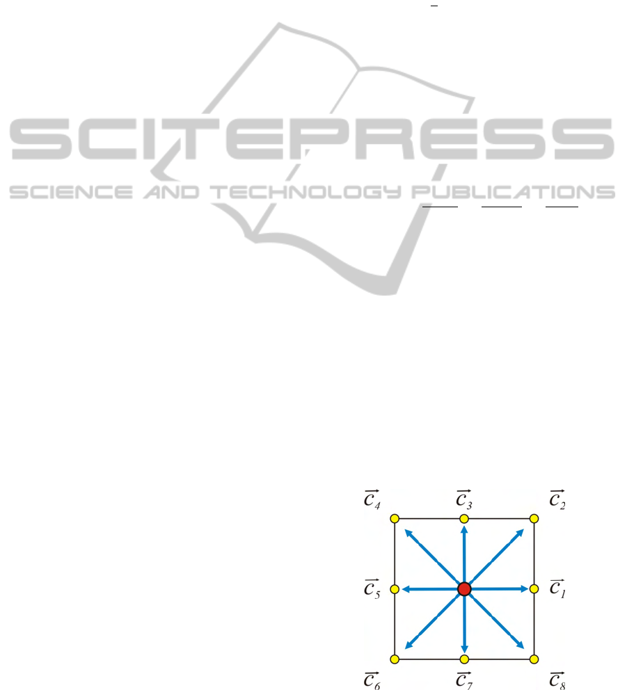
) respectively. In this work, our proposal is to
implement a two-dimensional LBM model, known
as D2Q9, which has 8 possibilities of non-zero
velocities, as shown in Figure 1.
The weights for the D2Q9 LBM model are given
Figure 1: The D2Q9 LBM node, with 8 non-zero velocities.
GRAPP 2012 - International Conference on Computer Graphics Theory and Applications
330

by:
ω
0
=
4
9
, ω
1,3,5,7
=
1
9
, ω
2,4,6,8
=
1
36
, (4)
where ω
0
is related to the rest particle. Replacing (4)
in (3), gives us the equilibrium function for the D2Q9
LBM model:
f
eq
i
= ω
i
ρ+ρ
0
3
(~c
i
·~u)
v
2
+
9
2
(~c
i
·~u)
2
v
4
−
3
2
(~u ·~u)
v
2
,
(5)
with i = 0,...,8. Our interest relies on the macro-
scopic scale, where the physical macroscopic quan-
tities seem to show a continuous behavior. Then, the
macroscopic density (ρ) and velocity (~u) are calcu-
lated from the respective moments of the density dis-
tribution, as follows:
ρ(~x,t) =
8
∑
i=0
f
i
(~x,t), (6)
~u(~x,t) =
1
ρ(~x,t)
8
∑
i=0
f
i
(~x,t)~c
i
. (7)
To compute the evolution of the simulation it is
need to define an initial configuration for the LBM
nodes such as the boundary condition. The initial con-
dition is defined for all the LBM nodes using the equi-
librium function given by expression (5). To do so, it
is necessary to set an initial value for the macroscopic
quantities (density and velocity). As will be explained
in section 6, the proposal of this work is to use a ve-
locity field computed by GVF as initial condition to
LBM.
Different types of boundaries have been intro-
duced in the field of hydrodynamics for the LBM.
Bounce-back is the simplest one, where boundary
nodes are placed halfway between the lattice nodes.
When the particles propagate to the boundary nodes,
they just bounce back along the direction they came
from. Due to its simplicity, this method does not
properly determine the velocity and density value for
these boundary nodes. An incorrect density or veloc-
ity value at the boundary nodes can eventually cause a
negative density value at local lattice points, and this
error can then accumulate along the simulation.
We implemented the boundary conditions based
on the work of (Zou and He, 1997), where the authors
proposed a way to specify density or velocity at the
boundary nodes, based on the idea of bounce-back of
the nonequilibrium distribution. To do so, we had to
take care of two kinds of boundary conditions: the
nodes that lie in the wall and the nodes that lie in the
corner of the lattice. In this approach, the boundary is
part of the simulation domain and a regular collision
is applied on boundary nodes.
4 THE GVF METHODOLOGY
The Gradient Vector Flow (GVF) field is defined as
the vector field v(x, y) = (u(x,y),v(x,y)) that mini-
mizes the energy functional:
ε =
Z Z
[µ(u
2
x
+ u
2
y
+ v
2
x
+ v
2
y
) + |F|
2
|v − F|
2
]dxdy
(8)
where F = (F
1
(x,y),F
2
(x,y)) is a field defined over
the domain of interest. When F is small, the energy
is dominated by partial derivatives of the vector field,
yielding a smooth field. Otherwise, the second term
dominates the integrand, and is minimized by setting
v = F. The parameter µ is a regularization parameter
that should be set according to degree of smoothness
required.
The GVF can be found by solving the associated
Euler-Lagrange equations given by:
µ∇
2
u − (u − F
1
)(F
2
1
+ F
2
2
) = 0 (9)
µ∇
2
v − (v − F
2
)(F
2
1
+ F
2
2
) = 0 (10)
where ∇
2
is the Laplacian operator. Equations (9) and
(10) can be solved by treating u and v as functions of
time t and solving:
u
t
(x,y,t) = µ∇
2
u(x,y,t) − (u(x, y,t) − F
1
(x,y))
·(F
2
1
+ F
2
2
) (11)
v
t
(x,y,t) = µ∇
2
v(x,y,t) − (v(x, y,t) − F
2
(x,y))
·(F
2
1
+ F
2
2
) (12)
subject to some initial condition v(x, y,0) = v
0
(x,y).
The steady-state solution (as t → ∞) of these parabolic
equations is the desired solution of the Euler-
Lagrange equations (9) and (10). These are reaction-
diffusion equations and are known to arise in areas
as heat conduction, reactor physics, and fluid flow.
The field obtained by solving the above equation is
a smooth and extended version of the original one.
5 SKETCH-BASED MODELING
The Sketch-Based Modeling (SBM) is a computa-
tional research area that focus on intuitive simplified
modeling techniques. It is based on the sketch process
made by traditional artist. Basically, the sketch-based
modeling program has to provide a comfortable and
intuitive environment where the artist can freely draw
his object. Then, using the sketch as an input, the pro-
gram must interpret the data and find an approximate
representation (Cook and Agah, 2009).
SKETCHING FLUID FLOWS - Combining Sketch-based Techniques and Gradient Vector Flow for Lattice-Boltzmann
Initialization
331

The sketch process starts with the drawing done
by the user through some input device (for example,
mouse, tablet or touch screen). This drawing is then
sampled and stored with some information such as
position, velocity, pressure, among others. The type
of information that can be stored depends on the de-
vice being used. For example, some devices provide
pressure information, multiple touches or slope of the
pen. Another device-dependent aspect is the sam-
ple frequency, which determines the sample distribu-
tion (Cruz and Velho, 2010).
The goal of a sketch-based modeling program is
to model the object intended by the user, not neces-
sarily what was drawn on the input device. One issue
with this type of system occurs when the user does
not have much ability to design or handling the de-
vice. In this case, the tracing performed may be in-
accurate. Another common issue is the noise from
the device, which comes from an inaccurate drawing
capture. Due to the presence of noise, it is common
to perform a filtering of sampled data. Another fea-
ture is to perform a fitting of the data for a convenient
curve (Cruz and Velho, 2010).
The data are stored as a sequence of points, T =
{p
1
,..., p
n
}, where n is the number of samples and
p
i
= (x
i
,y
i
,t
i
) indicates the position (x
i
,y
i
) and in-
stant t
i
each point was sampled. If the data acquisi-
tion device captures more information, the point can
be thought of as (x
1
,..., x
k
), where each element rep-
resents an attribute of the point. Besides the attributes
captured, it is also possible to calculate a few others,
such as velocity and acceleration. All this information
can be useful to add features to the model.
The points are conveniently grouped together to
build a two-dimensional model to which the system
must infer some meaning. This model is called the
sketch. The sketch can be used both for creating and
editing of 3D graphic object being modeled, such as
to control. In the latter case the application decides
which task to perform, according to the interpreta-
tion of the sketch. This is known as sketch of ges-
ture (Thorne et al., 2004).
6 PROPOSED METHOD
For modeling a fluid through LBM we need to dis-
cretize the domain, set the initial and boundary con-
ditions and then to apply the local rule of evolu-
tion. However, in the field of animation, it is com-
mon to generate scenes from advanced states of fluid
dynamics generated through fluid simulation tech-
niques. The initialization of the simulation is a fun-
damental step.
The main goal of this work is primarily concerned
with how to take drawing input from the user and con-
vert it into an initial fluid configuration. We claim
that such task can be implemented through an intu-
itive framework for fluid modeling using sketching
techniques and GVF. From the viewpoint of computer
graphics applications we need an efficient way to get
user actions, convert then into a model and to visual-
ize the model simulation.
In the case of fluid dynamics the sketching of the
initial configuration is much more complex because
there are too many degrees of freedom to consider.
However, in terms of high level features, the initializa-
tion of the LBM simulation can be performed through
the initial velocity field and convenient boundary con-
ditions that define the fluid behavior nearby the fron-
tiers of the domain.
In this work the main focus is a sketch based
framework to define the initial velocity field of the
fluid. In this way, streamlines are very intuitive fluid
features that can be mathematically defined by the ini-
tial value problem:
dx
dt
= v(x), x(0) = P
0
, (13)
where v, is the velocity field. The solution of this
problem for a set of initial conditions gives a set of
(integral) curves which can be interpreted as the tra-
jectory of massless particles upon the flow defined by
the velocity field.
Obviously the application of the mathematical
definition above only works if we know the veloc-
ity field which is exactly the target of our framework.
However, the streamline concept can be used as a
guide in the process of taking input drawings from the
user and to convert them into a model. Specifically,
once defined the boundaries of the fluid domain, the
user must draw a set of paths by moving the mouse
cursor that the system translates as streamlines. So,
the tangent field over these paths will be used to set
up the GVF computation in order to get the initial ve-
locity field.
The user paths are translated as streamlines of
the fluid and the corresponding tangent vector field
is computed. The tangent field computation can be
performed by fitting a spline model to each user path
or simply by taking a sequence of points p
1
,p
2
,..., p
k
over the path and computing the vectors v
i
= α
i
·
(p
i
− p
i−1
), i = 2, 3, ..., k, where α
i
is a scale factor
specified by the user in order to control the veloc-
ity field intensity over the streamline. A smoothed
version of the tangent field over these paths (convo-
lution with a Gaussian kernel) gives the field F =
(F
1
(x,y),F
2
(x,y)) in expressions (11)-(12) and the
initial condition v
0
of the GVF.
GRAPP 2012 - International Conference on Computer Graphics Theory and Applications
332
Then, the solution of GVF equations generates the
initial velocity field that we need to set up the LBM
simulation through the equilibrium function given by
expression (5).
To implement this idea, we shall provide an user
interface that allows free interaction for the user, as
we can see in Figure 2. In this figure we show a draw-
ing canvas aligned with the computer screen which
is used to define the fluid domain. The + and - but-
tons allow the user to change the domain resolution.
The SKETCH button makes possible for the user to
freely draw the sketching over the domain, using the
mouse. The HOLES button allows setting hole re-
gions into the fluid domain, which shall not be af-
fected by the fluid simulation model. The GVF button
takes the collection of points given by the sketch and
then compute the tangent field. After that, the tangent
field is used as input to the GVF method, which fi-
nally gives the initial velocity field that will be used as
input to the LBM. Finally, the RUN and RESET but-
tons control the simulation. The framework was de-
veloped using the C/C++ programming language with
the OpenGL library for the visualization.
For example, Figure 3(a) illustrates a sketching
made by the user in a 100 × 100 grid, with a hole in-
side the canvas defining a multiply connected domain.
The interface must interpret the user’s input and trans-
lates all the information to a fluid simulation model,
which shall recreate a visual state constrained to the
sketch. In this way, Figure 3(b) shows the tangent
field calculated along the sketching path, Figure 3(c)
Figure 2: The graphical user interface of the proposed
framework.
Figure 3: (a) Example of sketching made by the user. (b)
The tangent field. (c) The initial velocity field given by the
GVF. (d) The LBM initialization through the field in (c).
shows the velocity field given by the GVF using as in-
put the tangent field and respecting the multiply con-
nected domain. Finally, Figure 3(d) shows the initial-
ization of the LBM using the GVF as initial condition.
Such framework can be applied for 3D simula-
tions because all its basic components (GVF, LBM,
streamlines) are applied for three dimensional fields
without extra machinery.
7 RESULTS
In section 6 we explained our proposal for combining
sketch-based techniques and Gradient Vector Flow
for Lattice-Boltzmann initialization. This sections
presents some examples of fluid flows achieved by
our framework. For the results explained below the
dimension of the grid is 100 × 100.
The LBM initialization is given by the equilibrium
function defined in expression (5), which depends on
the macroscopic quantities density and velocity. The
initial macroscopic velocity field is given by the GVF
method. The initial macroscopic density field is de-
fined as ρ = 1.0. The experiments were performed
with an Intel Core 2 Quad 3.0 GHz, with 4 GB of
RAM and a Video Card NVidia GeForce 9800 GTX,
running Windows XP. The pictures in this article were
obtained through the implemented framework.
The first example defines a horizontal flow from
SKETCHING FLUID FLOWS - Combining Sketch-based Techniques and Gradient Vector Flow for Lattice-Boltzmann
Initialization
333
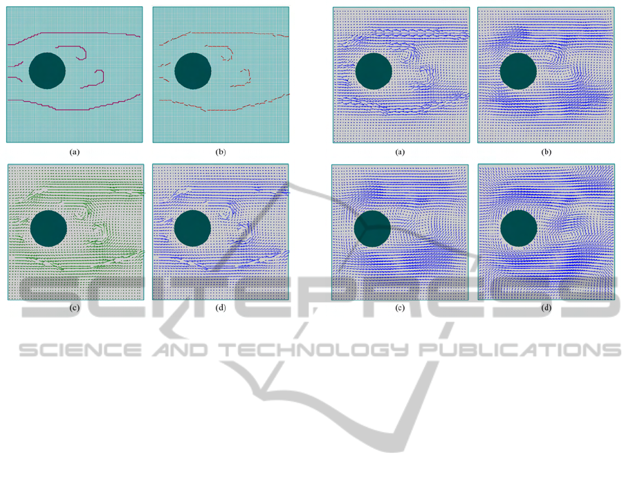
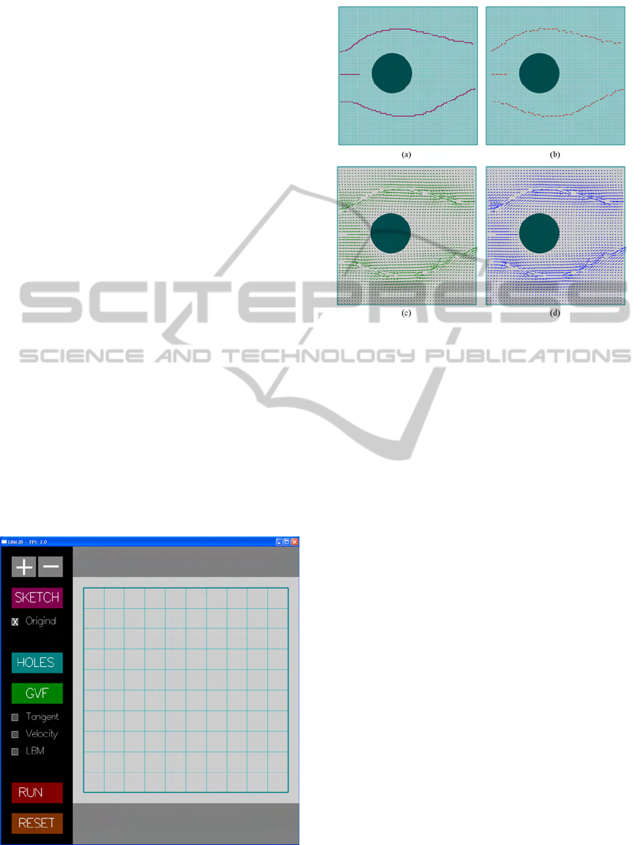
Figure 4: Example 1: horizontal flow from left to right with
a hole. (a) The sketching. (b) The tangent field. (c) The
initial velocity field given by the GVF. (d) The LBM initial-
ization through the field in (c).
left to right, with a hole in the domain. This exam-
ple shows a traditional 2D simulation of a flow past a
cylinder.
Figure 4(a) shows the sketching made by the user.
In Figure 4(b) we can see the tangent field calculated
through the sketching information. Once we have the
tangent field, the application is able to calculate the
GVF, shown in Figure 4(c).
Finally, the LBM is initialized using the GVF in-
formation as input, shown in Figure 4(d). In this case,
we expect some symmetry for the fields due to the
physics and geometry behind the fluid evolution. In
fact, we observe this property in the GVF result. The
Figure 5(a)-(d) illustrates four instants of the LBM
simulation for this example.
The next example illustrates a flow that happens
in the animation of a gas jet interacting with a solid
object. The sketching for this case is just a straight
line as shown in Figure 6(a). In Figure 6(b) we can
see the tangent field calculated through the sketching
information.
Once we have the tangent field, the application is
able to calculate the gradient vector flow, shown in
Figure 6(c). Finally, the LBM is initialized using the
GVF information as input, shown in Figure 6(d). We
can observe that the result of the gradient vector flow
gives the main stream of the jet, which is picture on
Figure 6(c).
After computing all these initial fields, we now
Figure 5: Example 1: the evolution of the fluid simulation.
The sequence (a)-(d) shows four instants of the LBM sim-
ulation, which was initialized using Figure 4(d) as initial
velocity condition.
are able to simulate the fluid which shall respect
our sketching. Figure 7(a)-(d) illustrates four in-
stants of the evolution of the fluid simulation through
LBM. We can observe that the LBM simulation can
reproduce the expected vortices in the surrounding
medium.
In the above examples the obstacles within the
fluid domain are fixed regions, where the velocity
field must be null. This is done automatically by
the system, through the mapping of the corresponding
LBM nodes. All these nodes are defined as a bound-
ary node.
Finally, the following example explores also the
flow past a cylinder starting from a sketching that is
a simplification of the flow shown in Figure 8. The
source of this figure is the work of (Schroeder et al.,
2010), which presents a sketch-based system to cre-
ate illustrative visualizations of 2D vector fields. This
figure pictures the illustrative visualizations of a snap-
shot of the flow when setting the Reynolds number to
100.
Our final example tries to simulate this behavior
through a simplified sketching. The Figure 9 pictures
a sketch of that flow representing a simplified version
of it, done through our framework. The Figure 10
shows the evolution of the simulation. We can ob-
serve that through a simplified sketching it is possible
to achieve approximate behaviors of complex flows.
GRAPP 2012 - International Conference on Computer Graphics Theory and Applications
334
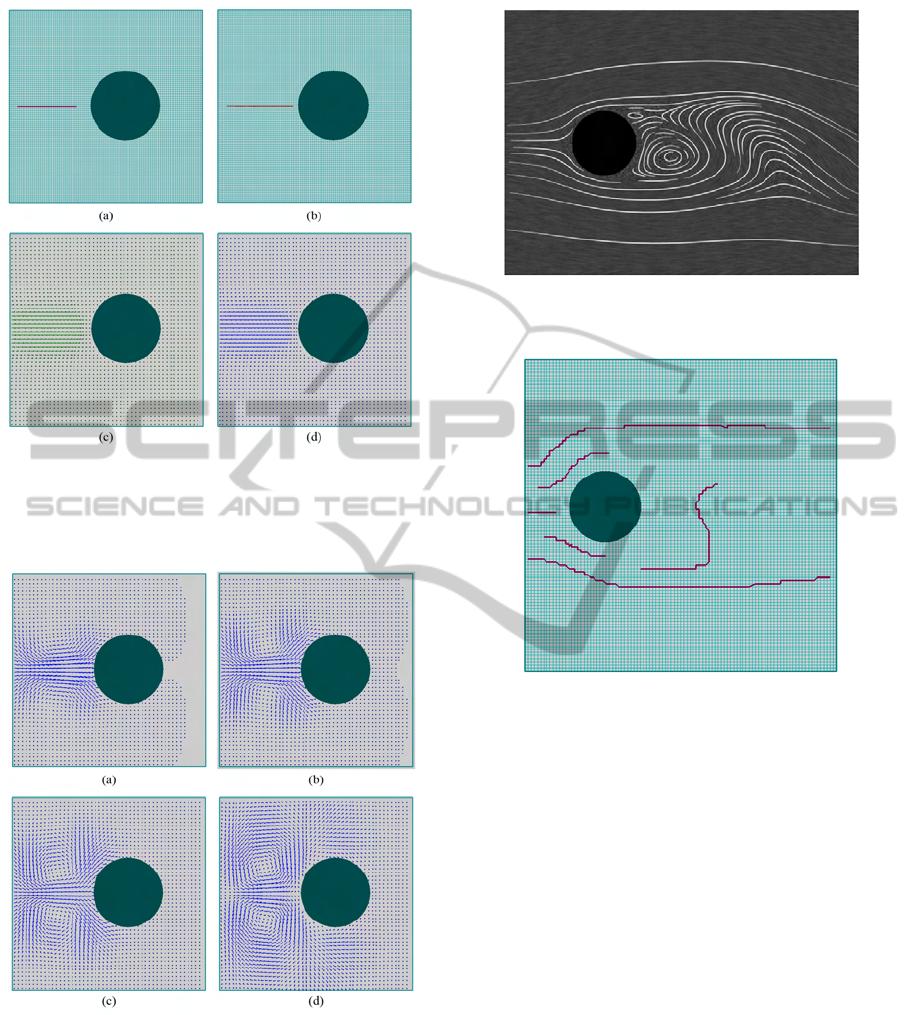
Figure 6: Example 2: flow of a gas with a solid object. (a)
The sketching. (b) The tangent field. (c) The initial velocity
field given by the GVF. (d) The LBM initialization through
the field in (c).
Figure 7: Example 2: the evolution of the fluid simulation.
The sequence (a)-(d) shows four instants of the LBM sim-
ulation, which was initialized using Figure 6(d) as initial
velocity condition.
8 CONCLUSIONS
In this work we presented a sketch-based system that
allows an intuitive fluid flow initialization for com-
Figure 8: An illustrative flow past a cylinder with Reynolds
number 100. (Source: (Schroeder et al., 2010))
Figure 9: A simplified version of the Figure 8.
puter graphics applications. We proposed a combina-
tion of sketching techniques with the Gradient Vec-
tor Flow method to obtain a smooth initialization for
the simulation. The fluid simulation is done using a
two-dimensional Lattice Boltzmann Method (LBM).
With the sketching techniques the system enables the
user to draw freely the initial state of the fluid flow
using an intuitive interface. The results section illus-
trates some classical examples of fluid flow simulated
through our system. We observed that it was able to
simulate some complex flows through simple initial
drawing.
A future direction for this work is to improve the
drawing process. Expected symmetries compose also
other point that our proposal must consider. For ex-
ample, in the 2D simulation of a flow past a cylinder
the animator is free to sketch a configuration which
does not have the symmetry observed in Navier-
Stokes simulations of incompressible flows with no-
slip boundary conditions. Our system must check
such problem and warn the user or automatically fix
it. The user is free to place the streamlines in any con-
figuration he has in mind. But, the user may sketch
SKETCHING FLUID FLOWS - Combining Sketch-based Techniques and Gradient Vector Flow for Lattice-Boltzmann
Initialization
335
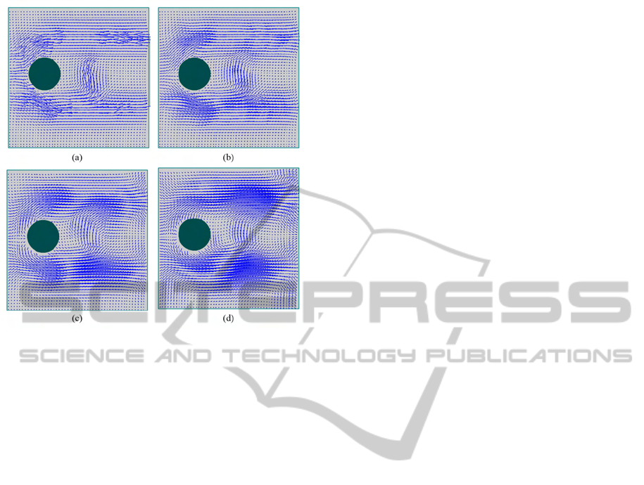
Figure 10: Example 3: the evolution of the fluid simulation.
unstable configurations that changes too fast without
adding extra machinery to the fluid flow model. This
may be an undesirable behavior depending on the an-
imator goals. Moreover, we want to combine image
processing techniques, so that we can use as input
some photos of fluid flows and extract from them a
potencial initial velocity field for the GVF method.
Another future direction of the proposed work is
to extend the two-dimensional approach to a three-
dimensional one. Such framework can be applied
for 3D simulations because all its basic compo-
nents (GVF, LBM, streamlines) are applied for three-
dimensional fields without extra machinery.
REFERENCES
Aubert, G. and Kornprobst, P. (2002). Mathematical Prob-
lems in Image Processing: Partial Differential Equa-
tions and the Calculus of Variations. Springer-Verlag,
New York.
Bærentzen, J. A. and Christensen, N. J. (2002). Volume
sculpting using the level-set method. In Proceedings
of the Shape Modeling International 2002 (SMI’02),
pages 175–, Washington, DC, USA. IEEE Computer
Society.
Buick, J. M., Easson, W. J., and Greated, C. A. (1998). Nu-
merical simulation of internal gravity waves using a
lattice gas model. International Journal for Numeri-
cal Methods in Fluids, 26(6):657–676.
Chen, S. and Doolen, G. D. (1998). Lattice boltzmann
method for fluid flows. Annual Review of Fluid Me-
chanics, 30:329–364.
Chopard, B., Luthi, P., and Masselot, A. (1998). Cellular
automata and lattice boltzmann techniques: An ap-
proach to model and simulate complex systems. In
Advances in Physics.
Cook, M. T. and Agah, A. (2009). A survey of sketch-based
3-d modeling techniques. Interact. Comput., 21:201–
211.
Cruz, L. and Velho, L. (2010). A sketch on sketch-based in-
terfaces and modeling. In Graphics, Patterns and Im-
ages Tutorials (SIBGRAPI-T), 2010 23rd SIBGRAPI
Conference on, pages 22 –33.
Foster, N. and Metaxas, D. (1997). Modeling the motion of
a hot, turbulent gas. In SIGGRAPH, pages 181–188.
ACM.
Higuera, F. J., Jimenez, J., and Succi, S. (1989). Boltzmann
approach to lattice gas simulations. Europhys. Lett.,
9.
Igarashi, T., Matsuoka, S., and Tanaka, H. (2007). Teddy: a
sketching interface for 3d freeform design. In ACM
SIGGRAPH 2007 courses, SIGGRAPH ’07, New
York, NY, USA. ACM.
McNamara, G. R. and Zanetti, G. (1988). Use of the boltz-
mann equation to simulate lattice-gas automata. Phys.
Rev. Lett., 61(20):2332–2335.
M
¨
uller, M., Keiser, R., Nealen, A., Pauly, M., Gross, M.,
and Alexa, M. (2004a). Point based animation of
elastic, plastic and melting objects. In ACM SIG-
GRAPH/Eurographics symposium on Computer ani-
mation, pages 141–151. Eurographics Association.
M
¨
uller, M., Schirm, S., and Teschner, M. (2004b). Inter-
active blood simulation for virtual surgery based on
smoothed particle hydrodynamics. Technol. Health
Care, 12(1):25–31.
Rothman, D. H. and Zaleski, S. (1994). Lattice-gas mod-
els of phase separation: Interface, phase transition and
multiphase flows. Rev. Mod. Phys, 66:1417–1479.
Schroeder, D., Coffey, D., and Keefe, D. (2010). Draw-
ing with the flow: a sketch-based interface for illustra-
tive visualization of 2d vector fields. In Proceedings
of the Seventh Sketch-Based Interfaces and Modeling
Symposium, SBIM ’10, pages 49–56, Aire-la-Ville,
Switzerland, Switzerland. Eurographics Association.
Stam, J. (2003). Flows on surfaces of arbitrary topology. In
SIGGRAPH, pages 724–731. ACM.
Sutherland, I. E. (1964). Sketchpad - a man-machine graph-
ical communication system. In Proceedings of the
SHARE design automation workshop, DAC ’64, pages
6.329–6.346, New York, NY, USA. ACM.
Thorne, M., Burke, D., and van de Panne, M. (2004). Mo-
tion doodles: an interface for sketching character mo-
tion. ACM Trans. Graph., 23:424–431.
Varley, P. A. C., Martin, R. R., and Suzuki, H. (2004). Can
machines interpret line drawings? EUROGRAPHICS
Workshop on Sketch-Based Interfaces and Modeling.
Wei, X., Member, S., Li, W., Mueller, K., and Kaufman,
A. E. (2004). The lattice-boltzmann method for sim-
ulating gaseous phenomena. IEEE Transactions on
Visualization and Computer Graphics, 10:164–176.
GRAPP 2012 - International Conference on Computer Graphics Theory and Applications
336

Williams, L. (1990). 3d paint. SIGGRAPH Comput. Graph.,
24:225–233.
Witting, P. (1999). Computational fluid dynamics in a tra-
ditional animation enviroment. In SIGGRAPH, pages
129–136. ACM.
Xu, C. and Prince, J. L. (1997). Gradient vector flow: A
new external force for snakes. In IEEE Proc. Conf.
On, pages 66–71.
Xu, C. and Prince, J. L. (1998). Snakes, shapes, and gradi-
ent vector flow. IEEE TRANSACTIONS ON IMAGE
PROCESSING, 7(3):359–369.
Zeleznik, R. C., Herndon, K. P., and Hughes, J. F. (2006).
Sketch: an interface for sketching 3d scenes. In ACM
SIGGRAPH 2006 Courses, SIGGRAPH ’06, New
York, NY, USA. ACM.
Zhu, B., Iwata, M., Haraguchi, R., Ashihara, T., Umetani,
N., Igarashi, T., and Nakazawa, K. (2011). Sketch-
based dynamic illustration of fluid systems. In SIG-
GRAPH ASIA 2011 Technical Papers, Hong Kong.
Zou, Q. and He, X. (1997). On pressure and velocity bound-
ary conditions for the lattice boltzmann bgk model.
Physics of Fluids, 9(6):1591–1598.
SKETCHING FLUID FLOWS - Combining Sketch-based Techniques and Gradient Vector Flow for Lattice-Boltzmann
Initialization
337
