
FEATURE-DRIVEN MAXIMALLY STABLE EXTREMAL REGIONS
P. Martins
1
, C. Gatta
2,3
and P. Carvalho
1
1
Centre for Informatics and Systems (CISUC), University of Coimbra, Coimbra, Portugal
2
Computer Vision Center, Autonomous University of Barcelona, Barcelona, Spain
3
University of Barcelona, Barcelona, Spain
Keywords:
Local Feature Detection, Maximally Stable Extremal Regions, Completeness.
Abstract:
The high repeatability of Maximally Stable Extremal Regions (MSERs) on structured images along with their
suitability to be combined with either photometric or shape descriptors to solve image matching problems have
contributed to establish the MSER detector as one of the most prominent affine covariant detectors. However,
the so-called affine covariance that characterizes MSERs relies on the assumption that objects possess smooth
boundaries, a premiss that is not always valid. We introduce an alternative domain for MSER detection
in which boundary-related features are highlighted and simultaneously delineated under smooth transitions.
Detection results on common benchmarks show improvements that are discussed.
1 INTRODUCTION
Vision tasks such as object recognition, view match-
ing, and tracking, just to name a few, are often per-
formed under the use of local descriptors, which are
usually characterized by an invariant response to cer-
tain classes of image transformations. A common
procedure to obtain the invariant description consists
in a preliminary detection of local image regions in a
covariant way, which will provide local patches to be
described in an invariant manner.
In the particular case of affine transformations, the
vision community has been prolific in introducing co-
variant feature detectors as well as invariant descrip-
tors. Detectors such as the Harris-Affine, Hessian-
Affine (Mikolajczyk and Schmid, 2004) or the Max-
imally Stable Extremal Regions (MSERs) algorithm
(Matas et al., 2002) are noteworthy solutions to detect
affine covariant features. For a complete review and
extensive references on this class of regions, we refer
the reader to the work of Tuytelaars and Mikolajczyk
(2008) and references within.
The almost linear complexity of the algorithm,
the repeatable results and the suitability of MSER
to be described by photometric or shape descriptors
(Moreels and Pietro, 2007; Forssen and Lowe, 2007)
have made the MSER detector one of the popular ref-
erences in the literature. Here, we bring into the anal-
ysis the well-known and not so well-known shortcom-
ings of the above mentioned detection. As a result,
we suggest an alternative domain for the detection of
MSERs which will allows us to retrieve a substan-
tially higher number of features and improve the ro-
bustness to blur. Furthermore, the new domain pro-
vides a more reliable summary of relevant image con-
tent via MSERs detection.
2 BACKGROUND AND
MOTIVATION
Before laying out a detailed description of the motiva-
tion behind our study, we will shortly review the basic
concepts and terminology around MSER detection.
2.1 Maximally Stable Extremal Regions
Concisely, a MSER is defined as an affine covariant
image region which is either brighter or darker than
its immediate surroundings and without any particular
shape. For a more formal definition, let us consider an
image as a mapping I : D → [0, 1], where D ⊂ R
2
. Let
us also denote the interior and the boundary of a con-
nected componentQ
c
in D as ∂Q
c
and int(Q
c
), respec-
tively. MSERs correspond to a very specific subset of
connected components in the image domain. They are
said to be extremal because the corresponding pixels
have either higher or lower intensity than all the pix-
els on its boundary: I |
int(Q
c
)
> c or I |
int(Q
c
)
< c for a
490
Martins P., Gatta C. and Carvalho P..
FEATURE-DRIVEN MAXIMALLY STABLE EXTREMAL REGIONS.
DOI: 10.5220/0003869204900497
In Proceedings of the International Conference on Computer Vision Theory and Applications (VISAPP-2012), pages 490-497
ISBN: 978-989-8565-03-7
Copyright
c
2012 SCITEPRESS (Science and Technology Publications, Lda.)
given c ∈ [0, 1], which is the value on the boundary.
Thus, Q
c
represents a maximal connected component
of a level set. Designating the region as stable refers
to the fact that a change of c = c + ∆, with ∆ > 0,
will imply minor changes in the area of the extremal
region. Q
c
will be coined as maximally stable if the
stability measure
ρ(Q
c
) =
|Q
c
|
d
dc
|Q
c
|
(1)
attains a local maximum at c (Matas et al., 2002; Kim-
mel et al., 2011).
2.2 MSER Detection: Known
Shortcomings
Probably, the most important property of MSER is its
affine covariance that can be directly inferred from
the covariance of the image level sets with respect to
affine transformations in the image domain. On the
other hand, the affine invariance of the detector’s sta-
bility measure guarantees the affine covariance of the
regions. However, as addressed and shown by Kim-
mel et al. (2011), the aforementioned property pre-
vails only if the boundaries of objects are smooth,
which is not always the case. Additionally, the strat-
egy adopted for the detection of these local features
is based on the assumption that images possess well-
defined structures (MSER features are usually an-
chored on region boundaries (Tuytelaars and Miko-
lajczyk, 2008)). These shortcomings have been re-
ported in the well-known comparative study on affine
covariant features performed by Mikolajczyk et al.
(2005). MSERs – along with Hessian-Affine regions
– have shown to be the most repeatable features in
the overall benchmark. However, the former has evi-
denced an expected less consistent behavior: reason-
ably textured scenes or blurred sequences were prone
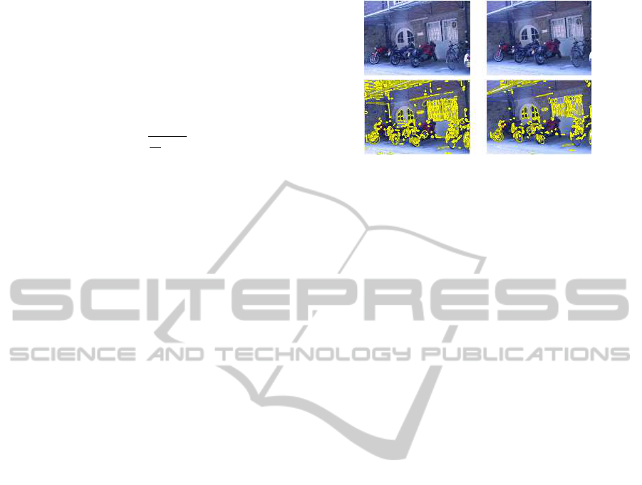
to provide less repeatable results. As an example,
Figure 1 illustrates such fragility when a progressive
de-focus blur is present: as it increases, the shape of
MSERs tends to change and, simultaneously, its num-
ber decreases.
Furthermore, the number of features that the
MSER detector retrieves is usually low if we compare
it to the number of local features detected by other
prominent detectors, e.g., Hessian-Affine or Harris-
Affine. We can regard this fact as a shortcoming of
MSER detection, as it might hinder the robustness of
MSERs to occlusions.
A quite less trivial but noteworthy characteristic
of MSER detection derives from the stability mea-
sure (Eq. (1)), which prefers round shapes to irreg-
ular ones. To our knowledge, Kimmel et al. (2011)
Figure 1: MSER detection (bottom row) on the first two
images of the “Bikes” sequence (top row). MSERs are rep-
resented by fitted ellipses.
have been the only ones to address the biased pref-
erence for regular shapes. In their paper, the authors
have illustrated this bias by showing that if two re-
gions have the same area and the same intensity along
their boundaries, the measure ρ tends to prefer the one
with a shorter boundary (perimeter). We emphasize
the importance of such property as most scenes con-
tain irregular shapes and we surely cannot claim that
regular shapes are always more distinctive than irreg-
ular ones.
2.3 Related Work: Other MSERs
We have highlighted some of the most important
shortcomings of MSER detection, namely (i) a rela-
tively high sensitivity to blurring, (ii) a small number
of features, and (iii) the preference of the algorithm
towards regular shapes.
A straightforward approach to reduce the sensitiv-
ity of MSER detection to blur is to apply a low-pass
filter to the input image. Such pre-processing will en-
hance the repeatability of MSERs in the presence of
blurred scenes, whereas the number of features will
be reduced. A more reliable alternative is to make
use of a multi-resolution detection: Forssen and Lowe
(2007) suggest an improved version of the MSER de-
tector by building a scale pyramid with one octave
between scales. MSERs are detected at each resolu-
tion and duplicated features at consecutive scales are
removed by comparing their locations. This strategy
leads to a higher number of detected features and an
improved repeatability under blur and scale changes.
However, it requires MSER features to be detected
at each resolution, which increases the computational
complexity of the method.
With the aim of freeing the MSER detector from
the existent preference towards round shapes, Kim-
mel et al. (2011) propose several reinterpretations of
the stability measure in order to define more informa-
tive shape descriptors.
FEATURE-DRIVEN MAXIMALLY STABLE EXTREMAL REGIONS
491

3 FEATURE-DRIVEN MSERS
We extend the concept of MSER to an alternative im-
age representation in which certain boundary-related
features are highlighted. MSERs detected on this do-
main will be coined as feature-driven MSERs. The
proposed domain is less sensitive to blurring and al-
lows the MSER detector to respond to a substantially
higher number of features per image. Moreover, ir-
regular shapes will appear more regular in the new
domain. In short, we propose a domain that encapsu-
lates the desired properties to yield a reliable MSER
detection, namely the existence of regular shapes and
well-defined boundaries combined with smooth tran-
sitions. The new domain is also designed to improve
the completeness of MSER features. We can regard
a set of features as a complete one if it preserves as
much as possible the information contained in the im-
age (Dickscheid et al., 2010). Increasing the number
of detected MSERs is not enough to produce a more
complete feature set; the regions should also preserve
the most relevant image content.
In the process of obtaining a domain characterized
by well-defined boundaries, but with smooth transi-
tions, we start by highlighting boundary-related fea-
tures. The process described herein highlights edges
using gradient information, which is a valid source
of information to build the domain with the desired
properties. Other alternatives can be considered for
feature highlighting, e.g., the eigenvalues of the Hes-
sian matrix.
For our purpose, obtaining smooth transitions at
the boundaries is as important as the process of fea-
ture highlighting and the consequent identification of
structural regions. The detection of structures at dif-
ferent scales will help us to define smooth transitions.
The process of averaging information over scales is
the key component to obtain the desired smoothness.
In the domain given as an example, we will highlight
edges and obtain smooth transitions by making use of
the gradient magnitude, computed by means of Gaus-
sian derivatives at several scales. Let L(:,σ) be the
result of convolving I with a Gaussian kernel g with
variance σ
2
. From the first order derivatives of L at
different scales, we obtain a new input for MSER de-
tection:
ˆ
L(~x) =
N
∑
i=1
σ
i
q
L
2
x
(~x,σ
i
) + L
2
y
(~x,σ
i
), (2)
where the standard deviation σ
i
varies in a geomet-
ric sequence σ
i
= σ
0
ξ
i−1
, with σ
0
∈ R
+
, ξ > 1, and
N denotes the number of scales. The final image is
the result of averaging gradient magnitude computed
at different scales. By doing this, with a reasonable
Bikes 1 Bikes 3
Input Images
Bikes 1:
ˆ
L(~x) Bikes 3:
ˆ
L(~x)
Feature highlighting
Feature-driven MSERS
Figure 2: Example of a detection of feature-driven MSERs
using the suggested domain. Detected features are repre-
sented by fitted ellipses.
number of scales, smooth transitions at the edges will
be obtained. Fig. 2 illustrates the suggested detec-
tion on a scene with de-focus blur. It is readily seen
that the new set of MSERs provides a good coverage
of the content and robustness to blur. The detection
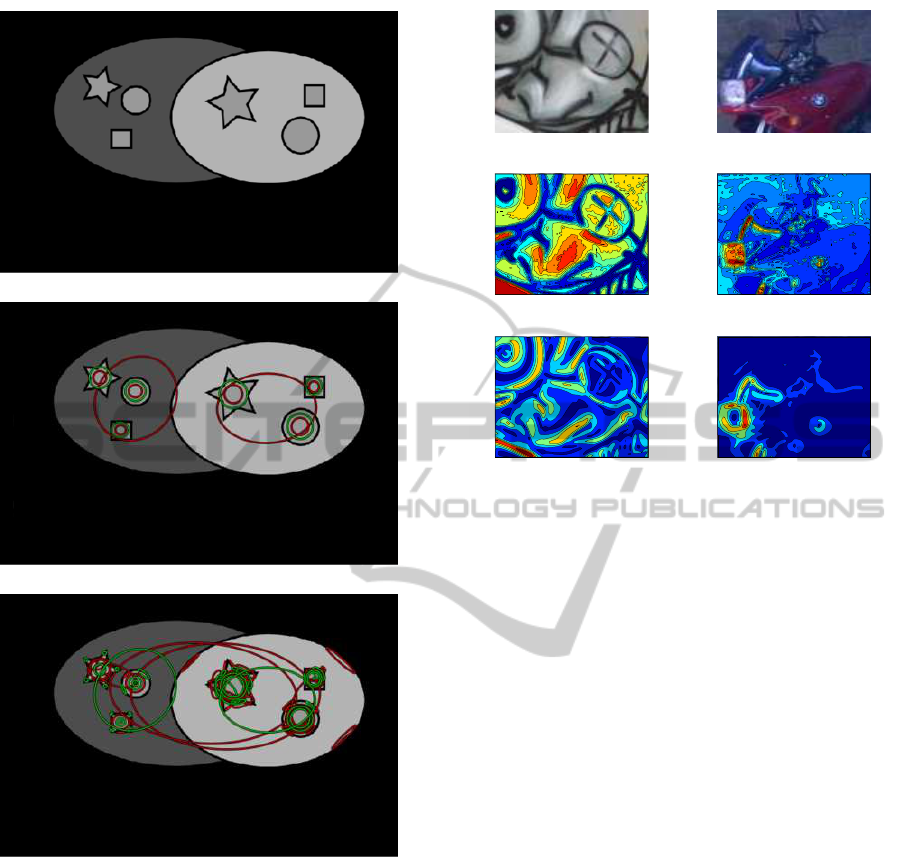
depicted in Fig. 3 serves as a more illustrative ex-
ample of the difference between original MSERs and
the proposed ones. For a better comprehension of the
proposed detection and due to the relatively low num-
ber of features detected on the synthetic image, we
distinguish in this example MSER+ features i.e., dark
regions with brighter boundaries, from MSER- fea-
tures, which correspond to bright regions with darker
boundaries. The latter features are obtained by giv-
ing the inverted image as input. As can be seen, the
use of the proposed domain yields a higher number
of MSERs. Furthermore, it allows us to capture in-
formative patterns in the scene such as corners and
junctions, which are usually neglected by a traditional
MSER detection.
The new domain will also attenuate the so-
called irregularity of extremal regions. Figure 4
helps to clearly illustrate the process of attenuation:
the boundaries of extremal regions correspond to
isophotes, i.e., iso-intensity countours. As expected,
these curves tend to appear irregular in shape on the
luminance channel (see Fig. 4-2(a)-(b)), whereas the
new domain providesmore regular shapes (see Fig. 4-
3 (a)-(b)). The examples in this figure equally demon-
strate that the proposed domain tends to highlight
relevant structures and present them as potential ex-
tremal regions. We can illustrate this fact with the
example of the logo on the motorbike: it appears as
a scattered object on the luminance channel, whereas
the new domain regards it as a relevant structure.
VISAPP 2012 - International Conference on Computer Vision Theory and Applications
492
(a)
(b)
(c)
Figure 3: MSER detection on a synthetic image (green:
MSER+, red: MSER-): (a) input image; (b) original de-
tection; (c) suggested detection.
4 EXPERIMENTAL VALIDATION
We have followed the guidelines given by the bench-
mark suggested by Mikolajczyk et al. (2005) to as-
sess the repeatability of the redefined MSER on pla-
nar scenes. In the literature, repeatability as been re-
garded as the fundamental criterion to assess the per-
formance of local features. Regardless of its impor-
tance, it does not provide a hint on the usefulness
and quality of the features. Therefore, our evalua-
tion has taken into account another important criterion
1 (a) 1 (b)
2 (a) 2 (b)
3 (a) 3 (b)
Figure 4: Isophotes and extremal regions: (1) input images;
(2) regions delineated by isophotes on the luminance chan-
nel; (3) regions delineated by isophotes on the suggested
domain.
that is often neglected: the completeness of features.
Furthermore, we would like to determine the level of
complementarity between MSERs extracted from the
original image and the proposed domain. Special em-
phasis is givento the performance of MSERs on struc-
tured images.
In this section, features that are retrieved using the
gradient-based image
ˆ
L as the input image for detec-
tion will be referred to as f-MSERs.
Implementation Details. We have made use of the
code provided by Vedaldi and Fulkerson (2008) for
MSER detection, which has been extended to deal
with images intensity values varying in a range dif-
ferent from {0, ... , 255}, as the new domain intensity
values might be greater than 255.
Parameter Settings. In the whole set of experi-
ments, the new domain was built with an initial scale
σ
2
0
= 0.64 and ξ = 1.19. N, the number of scales, was
set to 16. The default value for the variation param-
eter ∆ required by the stability measure is 10, as it is
a reasonably low number to give rise to a high num-
ber of features. The protocol that we have followed
evaluates the repeatability rate and the number of cor-
respondences. A less sparse detection often implies a
drop in the repeatability rate, albeit the potential in-
crease in the number of correspondences. For a reli-
FEATURE-DRIVEN MAXIMALLY STABLE EXTREMAL REGIONS
493
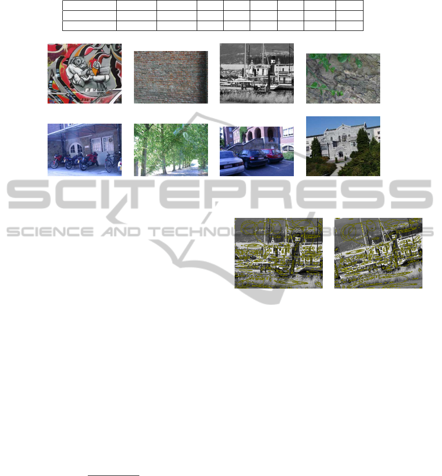
Table 1: Oxford dataset sequences.
Sequence Graffiti Wall Boat Bark Bikes Trees Leuven UBC
Texture X X X
Transformation Viewpoint Viewpoint Scale Scale Blur Blur Light JPEG
Graffiti Wall Boat Bark
Bikes Trees Leuven UBC
Figure 5: Oxford dataset sequences: example images.
able evaluation of these two criteria, detectors should
respond to a comparable number of features. Thus, in
some cases, we report results using additional values
for the variation parameter in the stability measure.
On one hand, the use of several ∆ allows us to have a
more insightful analysis and comparison of the main
results. On the other hand, it is also advantageous
to analyze results for a single (fixed) ∆: we can ex-
pect a higher number of f-MSER features but would
they be more repeatable than MSERs? Moreover, it
is interesting to assess the degree of complementarity
between MSER and f-MSER features when there is a
discrepancy between the cardinalities of sets.
4.1 Repeatability Evaluation
The benchmark suggested by Mikolajczyk et al.
(2005) computes the repeatability between regions
detected on two image pairs using 2D homographies
as a ground truth. Two regions are deemed as corre-
sponding and, therefore, repeated, with an overlap er-
ror of ε
0
× 100% if 1−
R
µ
1
∩R
(H
T
µ
2
H)
R
µ
1
∪R
(H
T
µ
2
H)
< ε
0
, where µ
1
and µ
2
denote the approximating ellipses of the two
detected regions, H is the homography and R
∗
repre-
sents the set of points identified by its subscript ∗. The
dataset, known as the Oxford dataset, comprises 8 se-
quences of images, each one with 6 images, whose
short description is outlined in Table 1 and depicted
in Fig. 5. One of the main motivations to define f-
MSERs is to find a more repeatable set of features in
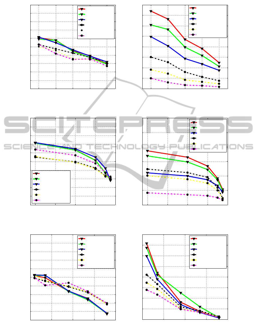
structured scenes, even when blur occurs. Figures 7
to 9 depict the repeatability and the correspondence
Figure 6: f-MSERs detected on the first and third images of
the “Boat” sequence.
plots for the sequences “Bikes”, “UBC” and “Boat”
(see detection results in Fig. 6), with an overlap er-
ror of 40%. The first image in each sequence is used
as the reference. In all the cases, it is clear that f-
MSER features are higher in number without show-
ing a significant drop in the repeatability rate. We
would like to stress that a substantially higher num-
ber of correspondences accompanied with a slight de-
crease of the repeatability rate is preferable to a minor
increase of the repeatability with less features, as in
the former the absolute number of repeated features
is considerably higher, which might provide a better
coverage of the content with a similar repeatability
rate. Nonetheless, the sequences of structured images
affected and corrupted by blur or JPEG compression
have shown an improved repeatability rate with the
use of f-MSERs. For the “Boat” sequence, we re-
port a decrease of the repeatability rate of f-MSERs
at higher scales. Nevertheless, the number of repeated
f-MSERs at higher scale changes is comparable to the
number of repeated MSERs.
For space reasons, we will not display all the re-
sults of the experiments in the form of plots. How-
ever, Table 2 gives a hint on the behavior of the de-
VISAPP 2012 - International Conference on Computer Vision Theory and Applications
494
2 3 4 5 6
0
10
20
30
40
50
60
70
80
90
100
Increasing blur
Repeatability (%)
2 3 4 5 6
0
200
400
600
800
1000
1200
1400
1600
Increasing blur
Number of correspondences
f−MSER (∆=10)
f−MSER (∆=20)
f−MSER (∆=50)
MSER (∆=10)
MSER (∆=20)
MSER (∆=50)
f−MSER (∆=10)
f−MSER (∆=20)
f−MSER (∆=50)
MSER (∆=10)
MSER (∆=20)
MSER (∆=50)
Figure 7: Repeatability rate and number of correspondences for the “Bikes” sequence (overlap error of 40%).
60 70 80 90 100
0
10
20
30
40
50
60
70
80
90
100
JPEG compression (%)
Repeatability (%)
60 70 80 90 100
0
500
1000
1500
2000
2500
3000
JPEG compression (%)
Number of correspondences
f−MSER (∆=10)
f−MSER (∆=20)
f−MSER (∆=50)
MSER (∆=10)
MSER (∆=20)
MSER (∆=50)
f−MSER (∆=10)
f−MSER (∆=20)
f−MSER (∆=50)
MSER (∆=10)
MSER (∆=20)
MSER (∆=50)
Figure 8: Repeatability rate and number of correspondences for the “UBC” sequence (overlap error of 40%).
1 1.5 2 2.5 3
0
10
20
30
40
50
60
70
80
90
100
Scale changes
Repeatability (%)
1 1.5 2 2.5 3
0
100
200
300
400
500
600
700
800
Scale changes
Number of correspondences
f−MSER (∆=10)
f−MSER (∆=20)
f−MSER (∆=50)
MSER (∆=10)
MSER (∆=20)
MSER (∆=50)
f−MSER (∆=10)
f−MSER (∆=20)
f−MSER (∆=50)
MSER (∆=10)
MSER (∆=20)
MSER (∆=50)
Figure 9: Repeatability rate and number of correspondences for the “Boat” sequence (overlap error of 40%).
tected regions for the complete dataset. It provides
the repeatability rate and number of correspondences
for the third image of each sequence as well as the cor-
responding average values for each sequence with an
FEATURE-DRIVEN MAXIMALLY STABLE EXTREMAL REGIONS
495

Table 2: Repeatability rate and number of correspondences
for each sequence (overlap error of 40%).
3rd image Sequence
(average)
MSER f-MSER MSER f-MSER
Grafitti 56%(310) 48%(538) 48%(244) 39%(402)
Wall 53%(2093) 57%(2484) 46% (1595) 46% (1786)
Boat 48%(658) 56%(861) 41%(388) 39%(556)
Bark 52%(276) 48%(355) 60% (268) 39%(295)
Bikes 47%(505) 58%(1328) 42%(360) 46%(1002)
Trees 38% (1767) 36% (1796) 33%(1295) 30%(1401)
Leuven 57%(668) 58%(901) 57% (488) 54%(768)
UBC 50%(1114) 63%(1647) 42% (825) 51%(1262)
overlap error of 40%. By analyzing the table, one can
conclude that feature-driven MSERs yield a consid-
erably higher number of correspondences. The lower
average repeatability rate of f-MSERs as seen in some
sequences is mainly due to the decrease of the re-
peatability rate in the last images of the sequence. As
theory confirms, in well-structured scenes, the new
MSERs can yield an increased repeatability. With re-
gard to sequences with viewpoint changes, f-MSERs
have shown a satisfactory repeatability. Nonetheless,
this repeatability can be improved if we build the do-
main under an affine scale-space.
4.2 Completeness Evaluation
How much of the image information is preserved
by local features? Feature sets should capture the
most relevant image content in order to provide
a trustworthy summarized description of the im-
age. This requirement is known in the literature
as completeness. A measure of completeness has
been proposed by Dickscheid et al. (2010). Suc-
cinctly, the incompleteness of a detection corresponds
to the following Hellinger distance: d(p
H
, p
c
) =
q
1
2
∑
~x∈D
(
p
p
H
(~x) −
p
p
c
(~x))
2
, where p
H
corre-
sponds to an entropy density, computed from local
image statistics and p
c
denotes a feature coding den-
sity, inferred from the set of features. We emphasize
that the completeness measure is not a simple way
of evaluating the image coverage of feature sets; it
penalizes local feature sets that contain less informa-
tive patterns despite of their coverage. For the pur-
pose of the evaluation, we defined a dataset compris-
ing images from the Oxford dataset sequences. Each
sequence was represented by its third image. The pa-
rameter settings for the detection coincide with the
ones used in the previous subsection. Table 3 outlines
the results of the completeness evaluation givenby the
Hellinger distance between the two aforementioned
distributions, using feature coding densities computed
from MSER and f-MSER feature sets as well as a
combination of both sets. The analysis of the latter
feature set results allows us to infer on the comple-
Table 3: Dissimilarity measure d(p
H
, p
c
) and number of
regions for the third image of each sequence.
MSER
MSER f-MSER f-MSER+ f-MSER- ∪
f-MSER
Graffiti 0.38(1085) 0.27(2216) 0.33(1130) 0.36(1086) 0.26
Wall 0.2(4433) 0.15(4981) 0.24(2711) 0.26(2270) 0.14
Boat 0.35(2319) 0.28(2720) 0.36 (1393) 0.35(1327) 0.27
Bark 0.29(1940) 0.19(2802) 0.27(1553) 0.31(1249) 0.18
Bikes 0.48(1123) 0.32(2388) 0.4(1311) 0.43(1077) 0.32
Trees 0.24(4821) 0.19(5299) 0.29(2529) 0.26(2770) 0.18
Leuven 0.45(1017) 0.36(1597) 0.44(869) 0.46(728) 0.35
UBC 0.29(2431) 0.26(2619) 0.35(1400) 0.35(1219) 0.24
mentarity of MSER and f-MSER features. Addition-
ally, we have analyzed the completeness of f-MSER+
and f-MSER- features. These results are summarized
in the same table.
It is important to note that MSER-like features are
not among the most complete ones (Dickscheid et al.,
2010). It is readily seen that homogeneous regions
are easily entitled to be classified as extremal regions,
which, in most of the cases, means excluding the most
informative content. Furthermore, the number of fea-
tures detected by the MSER algorithm tends to be
lower than the ones given by other prominent detec-
tors, such as the Hessian-Affine or the Harris-Affine.
One important conclusion to be drawn from Ta-
ble 3 is that f-MSER detection will provide us a
more complete set of features than the one comprised
of standard MSERs. The incompleteness values for
f-MSERs range from 0.15 (“Wall” image) to 0.36
(“Leuven” image), which reflects the high level of
completeness of these features. MSER features are
less complete and, in some cases, even less complete
than f-MSER+ or f-MSER- feature sets. The combi-
nation of MSER and f-MSERs features gives us the
most complete feature sets for each sequence. How-
ever, the complementary between both feature sets
is practically non-existent; the incompleteness values
for MSER ∪ f-MSER features are comparable to the
ones for feature-driven MSERs sets. This result helps
us to conclude that the relevant content preserved by
standard MSERs is also preserved by f-MSERs.
5 CONCLUSIONS AND FUTURE
RESEARCH DIRECTIONS
We have addressed the shortcomings of MSER detec-
tion as well as the desired properties of an image in
order to provide a reliable MSER detection. As result,
we have introduced an alternative domain for MSER
detection. This domain is mainly characterized by the
highlighting of certain boundary-related features and
the simultaneous presence of smooth transitions at the
boundaries. The detection of MSERs on this domain
responds to a higher number of regions than the one
VISAPP 2012 - International Conference on Computer Vision Theory and Applications
496

that uses the luminance channel as input. The feature-
driven MSERs tend to be more robust to blur than tra-
ditional ones. Furthermore, the new set of features
is more complete as it preserves more of the relevant
image content. The high level of completeness shown
by the feature-driven MSERs suggests that they can
be used to solve object recognition problems.
The new domain can be built with any func-
tion that responds to boundary-related features, which
gives several options to work with. In this paper, we
have used the gradient magnitude to build it and, as
future research directions, we intend to exploit other
measures to derive the domain. Future work also
includes assessing the performance of feature-driven
MSERs on object recognition problems.
REFERENCES
Dickscheid, T., Schindler, F., and F¨orstner, W. (2010). Cod-
ing images with local features. International Journal of
Computer Vision (in press).
Forssen, P.-E. and Lowe, D. (2007). Shape Descriptors for
Maximally Stable Extremal Regions. In Proc. of IEEE
11th Int. Conf. on Computer Vision, pages 1–8.
Kimmel, R., Zhang, C., Bronstein, A., and Bronstein, M.
(2011). Are MSER features really interesting? IEEE
Trans. on Pattern Analysis and Machine Intelligence,
33(11):2316–2320.
Matas, J., Chum, O., Urban, M., and Pajdla, T. (2002).
Robust wide baseline stereo from maximally stable ex-
tremal regions. In Proc. of the British Machine Vision
Conference 2002 (BMVC 2002), pages 384–393.
Mikolajczyk, K. and Schmid, C. (2004). Scale & affine
invariant interest point detectors. International Journal
of Computer Vision, 60(1):63–86.
Mikolajczyk, K., Tuytelaars, T., Schmid, C., Zisserman, A.,
Matas, J., Schaffalitzky, F., Kadir, T., and Gool, L. V.
(2005). A Comparison of Affine Region Detectors. In-
ternational Journal of Computer Vision, 65(1/2):43–72.
Moreels, P. and Pietro, P. (2007). Evaluation of Features
Detectors and Descriptors based on 3D Objects. Int. J.
Comput. Vision, 73(3):263–284.
Tuytelaars, T. and Mikolajczyk, K. (2008). Local invari-
ant feature detectors: a survey. Found. Trends Comput.
Graph. Vis., 3(3):177–280.
Vedaldi, A. and Fulkerson, B. (2008). VLFeat: An
open and portable library of computer vision algorithms.
http://www.vlfeat.org/.
FEATURE-DRIVEN MAXIMALLY STABLE EXTREMAL REGIONS
497
