3D RECONSTRUCTION OF PLANT ROOTS FROM MRI IMAGES
Hannes Schulz
1
, Johannes A. Postma
2
, Dagmar van Dusschoten
2
, Hanno Scharr
2
and Sven Behnke
1
1
Computer Science VI, Autonomous Intelligent Systems, University Bonn, Friedrich-Ebert-Allee 144, 53113 Bonn, Germany
2
IBG-2, Plant Sciences, Forschungszentrum J
¨
ulich, 52425 J
¨
ulich, Germany
Keywords:
Root Modeling, Plant Phenotyping, Roots in Soil, Maize, Barley.
Abstract:
We present a novel method for deriving a structural model of a plant root system from 3D Magnetic Resonance
Imaging (MRI) data of soil grown plants. The structural model allows calculation of physiologically relevant
parameters. Roughly speaking, MRI images show local water content of the investigated sample. The small,
local amounts of water in roots require a relatively high resolution, which results in low SNR images. However,
the spatial resolution of the MRI images remains coarse relative to the diameter of typical fine roots, causing
many gaps in the visible root system. To reconstruct the root structure, we propose a three step approach: 1)
detect tubular structures, 2) connect all pixels to the base of the root using Dijkstra’s algorithm, and 3) prune the
tree using two signal strength related thresholds. Dijkstra’s algorithm determines the shortest path of each voxel
to the base of the plant root, weighing the Euclidean distance measure by a multi-scale vesselness measure. As
a result, paths running within good root candidates are preferred over paths in bare soil. We test this method
using both virtually generated MRI images of Maize and real MRI images of Barley roots. In experiments on
synthetic data, we show limitations of our algorithm with regard to resolution and noise levels. In addition we
show how to use our reconstruction for root phenotyping on real MRI data of Barley roots in soil.
1 INTRODUCTION
In this paper, we present a method for deriving a struc-
tural model of plant roots from MRI measurements
of roots in soil (cmp. Fig. 1). From this model, we
then derive local root mass and diameter together with
suitable statistics.
Plant roots are ‘the hidden half’ of plants (Waisel
et al., 2002) because non-invasive root imaging in nat-
ural soils is hampered by a wide range of constrictions.
For a full, non-destructive 3D assessment of root struc-
ture, topology and growth, only two main techniques
are currently available, Computer Tomography, using
X-Rays or neutron (Nakanishi et al., 2003; Pierret
et al., 2003; Ferreira et al., 2010) and Nuclear Mag-
netic Resonance Imaging (MRI) (Brown et al., 1990;
Southon and Jones, 1992; Jahnke et al., 2009). Both
X-ray CT and MRI are volumetric 3D imaging tech-
niques, where CT is based on absorption and MRI is
an emission-based technique.
For MRI, most signal stems from water in the roots
and to a lesser extend from soil water. Even though
MRI contrast can be adapted such that discrimination
between root water and soil water is maximized (see
Sec. 3), signal-to-noise ratio (SNR) remains relatively
low. In addition, contrast can be enhanced by manip-
Figure 1: A simulated maize root MRI image at SNR 150
(left) and its true and fitted structure model overlayed, with
missing/additional pieces marked in strong red/blue (right).
24
Schulz H., A. Postma J., van Dusschoten D., Scharr H. and Behnke S..
3D RECONSTRUCTION OF PLANT ROOTS FROM MRI IMAGES.
DOI: 10.5220/0003869800240033
In Proceedings of the International Conference on Computer Vision Theory and Applications (VISAPP-2012), pages 24-33
ISBN: 978-989-8565-04-4
Copyright
c
 2012 SCITEPRESS (Science and Technology Publications, Lda.)

ulating the soil mixture such that mainly signal from
the roots is detected.
With the same equipment, MRI measurements can
be done at different spatial resolutions, where lower
resolution results in a significant reduction in mea-
surement time. This is relevant for root phenotyping
studies, where larger quantities of plants need to be
measured repeatedly over a longer period. Thus, one
of our main concerns is in how far a diminishing res-
olution and low SNR reduces the accuracy of a root
reconstruction algorithm. For plant root studies, this
algorithm should produce from the MRI measurements
estimates for local and overall root mass, root length,
and diameter. Here, we examine the capability of a
novel root reconstruction algorithm to obtain these es-
timates at different image resolutions and noise levels.
As root diameters may be of subvoxel size, voxel-
wise segmentation would be brittle. We therefore re-
construct a structural, i. e. zero-diameter model of the
root system and subsequently derive parameters like lo-
cal root mass and diameter, without finding step edges
in the data. To construct the root structure, we first
find tubular structures on multiple scales. We then
determine the plant shoot position and connect every
root candidate element to it by a shortest path algo-
rithm. Finally, we prune the graph using two intuitive
thresholds, and adjust node positions with subvoxel
accuracy by a mean-shift procedure. For root mass and
diameter estimation, we use the scale value σ giving
maximum response of the (Frangi et al., 1998) tubular-
ness measure V (σ) (see Eq. 1). Root mass can then be
derived by locally summing image intensities within a
cylinder of the found diameter around the root center.
After reviewing related work, we start by giving a
short overview of the MRI method applied (Sec. 3), fol-
lowed by a description of the novel root reconstruction
algorithm (Sec. 4) and how to use the reconstructed
root to derive root statistics (Sec. 5). Experiments in
Sec. 6 demonstrate the performance of our approach.
2 RELATED WORK
Data similar to ours has been analyzed extensively in
the biomedical literature, e.g. using the multi-scale
“vesselness” measure of (Frangi et al., 1998). Of many
suggested approaches for finding and detecting ves-
sels, (Lo et al., 2010) is most similar to ours. Our
approach is less heuristic, however, and uses knowl-
edge of global connectedness. While the primary focus
of most approaches is visualization, we aim at fully
automated extraction of root statistics, such as length
and water distribution, to model roots and biological
processes of roots.
So far, only few image processing tools are avail-
able for plant root system analysis (Dowdy et al., 1998;
M
¨
uhlich et al., 2008; Armengaud et al., 2009). For
these tools, however, roots need to be well visible, e. g.
by invasively digging them out, washing, and scanning
them or by cultivating plants in transparent agar (Nagel
et al., 2006). Analysis is restricted to 2D data. Large
root gaps, artifacts due to low SNR, or reconstruction
in 3D have not yet been addressed.
Classical, non-invasive image-based root system
analysis tools in biological studies are e. g. 2D rhi-
zotrons (Pierret et al., 2003). 3D MRI has already been
used in root-soil-systems for the analysis of e. g. water-
flow (Haber-Pohlmeier et al., 2009). Semi-automated
reconstruction of roots by 3D CT based on a multi-
variate grey-scale analysis has recently been shown
to work (Tracy et al., 2010). However, to the best of
the authors knowledge, fully automatic root system
reconstruction in 3D data is new.
3 IMAGING ROOTS IN SOIL BY
MRI
MRI is an imaging technique well-known from med-
ical imaging and general background information is
available in textbooks, see e. g. (Haacke et al., 1999).
The MRI signal is proportional to the proton density
per unit volume, modulated by an NMR relaxation phe-
nomenon called T
2
relaxation. It causes an exponential
signal decrease after excitation that can be partially
refocused into an echo. Plant root analysis in soil was
so far hampered by a relatively poor contrast between
roots and surrounding soil water. However, soil wa-
ter contribution to the echo signal can be reduced to
less than 1%, increasing contrast significantly. This is
achieved by mixing small soil particles (a loamy sand)
and larger ones and keeping the water saturation of
the soil at moderate levels. Thus, the soil water T
2
(re-
laxation time) is only a few milliseconds whereas the
root water T
2
is several tens of milliseconds. Using an
echo time of 9 ms, the signal amplitude of soil water is
damped severely, whereas the root water signal inten-
sity is only mildly affected. Additionally, as magnetic
particles disturb MRI signals heavily, such particles
should be removed from the soil beforehand to assure
a high-fidelity 3D image reconstruction.
The MRI experiments were carried out on a verti-
cal 4.7 Tesla spectrometer equipped with 300 mT/m
gradients and a 100 mm r.f. coil (Varian, USA). 3D
images were generated using a so-called single echo
multi slice (SEMS) sequence, with a field of view
of 100 mm and a slice thickness of 1 mm. A barley
plant was grown in a 420 mm long 90 mm diameter
3D RECONSTRUCTION OF PLANT ROOTS FROM MRI IMAGES
25

Figure 2: Root diameter distribution of the root shown in
Figure 1.
PVC tube with a perforated bottom to prevent water
clogging. Measurements where performed about 6
weeks after germination. Because the tube is longer
than the homogeneous r.f. field, it was measured in
five stages. The resulting image stacks were stitched
together without any further corrections. The final
192 × 192 × 410 volumetric image has a lateral spatial
resolution of 0.5 mm and a vertical resolution of 1 mm.
3.1 Synthetic MRI Images
Synthetic MRI images were generated using SimRoot,
a functional-structural model capable of simulating the
architecture of plant roots (Postma and Lynch, 2011a;
Postma and Lynch, 2011b). Virtual root models of
15 day old maize plants
1
were converted into scalar
valued images in which the pixel value corresponds
to the root mass within the 0.5 mm cubed pixels. Five
images were generated from five runs, which only
varied due to variation in the model’s random number
generators. We added variable amounts of Gaussian
noise to the images at SNRs of 10, 50, 100, 150, 200,
and 500. Note that even images with high SNR cannot
simply be thresholded, since roots thinner than a voxel
would not be detected anymore. The resolution of the
images with SNR of 150, i. e. an achievable SNR in
real MRI data, were scaled down in the two horizontal
dimension to voxel dimensions of 0.5, 0.67, 1, and
1.3 mm to see how the resolution of the MRI image
might affect the results. Figure 1, left, shows one of
the simulated maize root images, and Figure 2 its root
diameter distribution. Please note, that as for real roots
not all diameters are populated in the histogram.
1
Barley plants are not yet available in SimRoot. 15 day
old maize roots come closest to the barley root data.
4 RECONSTRUCTION OF ROOT
STRUCTURE
We build a structural root model from volumetric MRI
measurements in four main steps. First, we find tubular
structures on multiple scales. Secondly, we determine
the shoot position (the horizontal position of the plant
at ground level). Thirdly, we use a shortest path algo-
rithm to determine connectivity. Finally, we prune the
graph using two intuitive thresholds.
Finding Tubular Structures. We follow the ap-
proach proposed by (Frangi et al., 1998), which is
widely used in practice. MRI images typically do
not contain isotropic voxels. The axes are therefore
first scaled up using cubic spline interpolation. The
result L(x) (Fig. 3(b)) is then convolved with a three-
dimensional isotropic derivative of a Gaussian filter
G(x,σ) . The standard deviation σ determines the scale
of the tubes we are interested in:
∂
∂x
L(x,σ) = σ
γ
L(x) ∗
∂
∂x
G(x,σ).
In the factor σ
γ
, introduced by (Lindeberg, 1996) for
fair comparison of scales, γ is set to 0.78 (for a tubular
root model as in (Krissian et al., 1998)). Differenti-
ating again yields the Hessian matrix H
o
(σ) for each
point x
o
of the image. The local second-order structure
captures contrast between inside and outside of tubes
at scale σ as well as the tube direction. Let λ
1
,λ
2
,λ
3
( |λ
1
| ≤ |λ
2
| ≤ |λ
3
| ) be the eigenvalues of H
o
(σ) . For
tubular structures in L holds: |λ
1
| ≈ 0 , |λ
1
|  |λ
2
| ,
and |λ
2
| ≈ |λ
3
| . The signs and magnitudes of all three
eigenvalues are combined in the medialness measure
V
o
(σ) proposed in (Frangi et al., 1998) (Fig. 3(c)),
determining how similar the local structure at x
o
is to
a tube at scale σ:
V
o
(σ) =



0 if λ
2
> 0 or λ
3
> 0

1−e
−λ
2
2
2α
2
λ
2
3

| {z }
R
A
e
−λ
2
1
2β
2
|λ
2
λ
3
|
| {z }
R
B

1−e
−
∑
i
λ
2
i
2c
2

| {z }
S
.
Here, R
A
distinguishes between plate-like and line-
like structures, R
B
is a measure of how similar the
local structure is to a blob, and S is larger in regions
with more contrast. The relative weight of these terms
is controlled by the parameters α and β , which we
both fixed at 0.5 . Finally, we combine the responses
of multiple scales by selecting the maximum response
V
o
= max
σ∈
{
σ
0
,...,σ
S
}
V
o
(σ). (1)
where σ
i
= (σ
S
/σ
0
)
i/S
· σ
0
. For our experiments, we
select σ
0
= 0.04 mm, σ
S
= 1.25 mm, and S = 20.
VISAPP 2012 - International Conference on Computer Vision Theory and Applications
26

Finding the Shoot Position. In our model, we uti-
lize the fact that plant roots have a tree graph structure.
The root node of this tree is a point at the base of the
plant shoot, which has, due to its high water content
and large diameter, a high intensity in the image. To
determine the position of the base of the plant shoot
x
r
, we find the maximum in the ground plane slice p
convolved with a Gaussian G(x,σ) with large σ,
x
r
= arg max
x
{
L(x,σ)|x
3
= p
}
.
Determining Connectivity. So far, we have a local
measure of vesselness V at each voxel and an initial
root position x
r
. What is lacking, is whether two neigh-
boring voxels are part of the same root segment and
how root segments are connected. In contrast to some
medical applications, we can use the knowledge of
global tree connectedness. For this purpose, we first
define a graph on the voxel grid, where the vertices
are the voxel centers and edges are inserted between
all voxels in a 26-neighborhood. We further define an
edge cost w for an edge between x
s
and x
t
as
w(x
s
,x
t
) = exp (−ω(V
s
+ V
t
))
with ω  0 . For each voxel x
o
, we search for the
minimum-cost path to x
r
. This can efficiently be done
using the Dijkstra algorithm (Dijkstra, 1959), which
yields a predecessor for each node in the voxel graph,
determining the connectivity.
Model Construction. Every voxel x
o
is now con-
nected to x
r
, but we already know that not all voxels
are part of the root structure. The voxel graph needs
to be pruned to represent only the roots. For this pur-
pose, it is sufficient to select leaf node candidates that
exceed the two thresholds explained below. The nodes
and edges on the path from leaf node x
l
to x
r
in the
voxel graph are then added to the root graph.
In a first step we cut away all voxels from the graph
with L(x) < L
min
, meaning that a leaf node candidate
needs to contain a minimum amount of water.
In a second step, we find leaf nodes of the tree,
i. e. root tips. To do so, we search for high values in
a median-based ‘upstream/downstream ratio’ D for
voxel x
o
D
o
= median
u∈N
+
m
(x
o
)
(L(u))/median
d∈N
−
m
(x
o
)
(L(d)),
where neighborhood N
−
m
(x
o
) denotes the m predeces-
sor voxels of x
0
with highest V when following the
graph for m steps away from x
r
(i. e. into the soil),
and N
+
m
(x
o
) are the m successor voxels with highest
V when following the graph for m steps towards x
r
(i. e. into the root). Thus, D
o
is approx. 1 for voxels
surrounded by soil and voxels lying in a root since
there, the only variations of L(x) are due to noise. D
o
is largest and in the range of SNR for voxels indicat-
ing a root tip as we encounter ‘signal’ on the one side
of the voxel and ‘noise’ on the other. Thus root tips
are voxels where D
o
> D
min
, where D
min
is a tuning
parameter.
In roots with large diameter, there are still multiple
paths from the outer rim to the root center. In a final
step, we remove segments which contain a leaf and are
shorter than the maximum root radius from the root
graph. This step is iterated as long as segments can be
removed from the graph.
5 ESTIMATION OF ROOT
PARAMETERS
In most biological contexts local and global parameters
describing the phenotype of a root are needed, e. g. to
derive species-specific models of roots. In this section,
we show how to derive such parameters supported by
our model.
Root Lengths. To determine the root lengths, high-
precision positioning of vertices is essential. So far,
vertices are positioned at voxel centers. We now apply
a mean-shift procedure to move the nodes to the center
of the root with subvoxel precision. At each node n at
position x
n
, we estimate the inertia tensor in a radius
of 3 mm and determine its eigenvalues λ
1
≤ λ
2
,≤ λ
3
as well as corresponding eigenvectors v
1
,v
2
,v
3
. If
λ
3
> 1.5λ
2
, we assume v
3
to correspond to the local
root direction. We then move the node to the mean
of a neighborhood in the voxel grid weighted by the
vesselness measure V (Eq. 1). To do so, we choose a 4-
neighborhood of x
n
in the plane spanned by v
1
and v
2
,
and evaluate V by linear interpolation. Nodes where
no main principal axis can be determined ( λ
3
< 1.5λ
2
)
are moved to the mean of their immediate neighbors in
the root graph. We iterate these steps until convergence.
The resulting structural model is shown in Fig. 3(a).
Finally, we can determine the total root lengths by
summing over all edge lengths.
Root Radius. For estimation of the local root radius
r(x) , we use the argument leading to the maximum
response V
o
in Eq. 1
r
o
= arg max
σ∈
{
σ
0
,...,σ
S
}
V
o
(σ) (2)
at location x
o
. The radius assigned to a node is calcu-
lated by averaging r in each segment. A root segment
is a list of all vertices connected to each other by ex-
actly two connections, meaning they are either ended
by a junction or a root tip.
3D RECONSTRUCTION OF PLANT ROOTS FROM MRI IMAGES
27

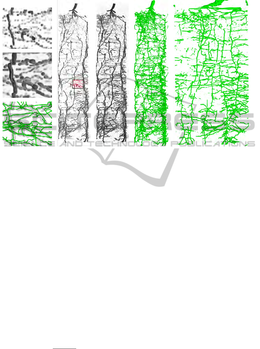
(a) (b) (c) (d) (e)
Figure 3: Root model reconstruction. ( a ) Raw data, tubeness-measure (Frangi et al., 1998), structural model. Volume rendering
of ( b ) raw data and ( c ) tubeness-measure. ( d ) 3D rendering of model, edges weighted by estimated diameter. ( e ) Cylindrical
projection of model.
Root Mass. Root mass is derived by sampling along
segments in 0.2 mm steps. We mark for each sampling
location x
o
all voxels within the local radius r
o
. The
mass of a root segment is the sum of values L of all
marked voxels.
For constant water density ρ in the roots the mass
of a root slice of length l can be calculated from its
radius and vice versa
m
o
= ρπr
2
o
l (3)
Thus especially for subvoxel roots mass estimate may
be used as a radius measure.
6 EXPERIMENTS
6.1 Synthetic Maize Roots
Of the five synthetic root systems, one root system is
set aside to tune the two thresholding parameters from
Sec. 4 so that they maximize the F
0.5
measure (van
Rijsbergen, 1979)
F
0.5
=
1.25P · R
0.25P + R
. (4)
with precision P and recall R . Precision P is the frac-
tion of true positives in all found positives (true and
false positives), while recall is the fraction of true pos-
itives in all elements that should have been found (true
positives and false negatives). The precision P has
double the weight of recall R in the F
0.5
measure in
order to reduce the chance of false positives. As a
result the chance of false negatives increases, however
this error is relatively small compared to the current
detection error of fine roots by the MRI.
To determine true/false positives and false nega-
tives for precision and recall, we sample synthetic and
reconstructed roots in 0.2 mm steps and determine the
closest edge of the respective other model. A ‘match’
occurs when this distance is smaller than one voxel
size.
6.2 Sensitivity to Resolution and Noise
For quantitative analysis of our reconstruction algo-
rithm, we use synthetic data of maize roots (see Sec. 3).
Fig. 4 shows a typical detail view of such data at
SNR 150. At this SNR Frangi’s tubularness mea-
sure (Eq. (1) , Fig. 4b) gives a reasonable indication of
where the root is. Figs. 4c, d show the found positions
before and after subvoxel positioning. In Fig. 4d we
VISAPP 2012 - International Conference on Computer Vision Theory and Applications
28

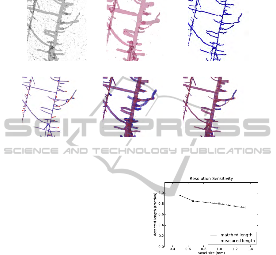
(a) (b) (c)
(d) (e) (f)
Figure 4: Example of a reconstructed root (detail): false positives, false negatives, and diameter estimates. ( a ) Raw data at SNR
150, ( b ) tubular structures enhanced using Eqn. (1) , ( c ) extracted structure model before subvoxel positioning, ( d ) true and
fitted structure model overlayed, with missing/additional pieces marked in strong red/blue, ( e ) diameter estimates, ( f ) mass
estimates.
see that most parts of the root system are correctly
detected, however, at junctions and crossings the algo-
rithm sometimes prefers shortcuts over the true root
path. For root length the effect has not much influence,
however branching angles are slightly biased towards
90
◦
. In addition, as short ( < 3 mm ) root elements are
suppressed for the sake of robustness with respect to
noise and uncorrect skeletonization of thick roots, true
short root elements are non-surprisingly missing.
Diameter and mass of the roots are shown in
Fig. 4e, f, where in Fig. 4e diameter is estimated from
the Frangi scales (Eq. 2), and in Fig. 4f diameter is cal-
culated from the estimated mass (by inverting Eq. 3).
We observe that radius from mass, i. e. from the mea-
sured image intensities, is much more reliable than the
geometry-based estimate—especially for smaller roots.
However, this is only possible under the assumption
of constant water density in the root, being perfectly
true for our synthetic data. While for healthy roots this
is also well fulfilled, the radius of drying roots will
unavoidably be systematically underestimated by this
method.
In the next sections we investigate the statistical
properties of the found root systems with respect to
root length, volume, and diameter.
6.2.1 Root Length
Data acquisition time for MRI scales with image reso-
Figure 5: Influence of image resolution: fraction of detected
overall root length versus voxel size, for five individual data
sets showing 15 day old maize roots at SNR 150. Matched
length indicates true positives only, measured length also
includes false positives.
lution. Therefore, image resolution should be selected
as low as possible with respect to the measurement
task at hand. In order to test sensitivity of our root
reconstruction algorithm with respect to image reso-
lution, we calculated root length from the synthetic
MRI data (see Sec. 3) with SNR = 150 and varying
image resolution and compared to the known ground
truth. Fig. 5 shows how detected root length decreases
with larger voxel sizes. For the highest resolution pro-
vided (0.5 mm), 95.5% of the true overall root length is
detected with standard deviation 0.3%, which is well
acceptable for most plant physiological studies.
3D RECONSTRUCTION OF PLANT ROOTS FROM MRI IMAGES
29

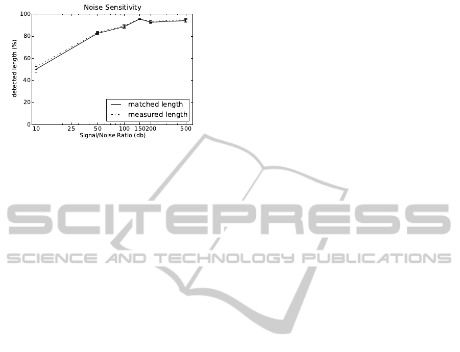
Figure 6: Influence of noise: fraction of detected overall
root length versus signal to noise ratio, for five individual
data sets showing 15 day old maize roots at 0.5 mm voxel
size. Matched length indicates true positives only, measured
length also includes false positives.
Increasing voxel size quickly decreases found root
length to 80% at 1 mm voxel size and to ≈ 72% at
1.33 mm voxel size. For larger voxels, false positives
have a measurable influence of about 2%. For high-
est resolutions, false positives have no significant in-
fluence. We conclude, that voxel size should not be
greater than 0.5 mm.
As with other imaging modes, SNR of MRI data
increases with acquisition time. Thus, to keep acqui-
sition time short, image noise should be selected as
high as possible with respect to the measurement task
at hand. We calculated root length from the synthetic
MRI data (see Sec. 3) with 0.5 mm voxel size and vary-
ing noise levels and compared to the known ground
truth (see Fig. 6). For the lowest SNR (10), only 50%
of the roots are detected. Detection rate quickly in-
creases with increasing SNR and levels off to 95% at
an SNR of about 150. At the given resolution, an SNR
of 150–200 seems to give the best balance between
detection accuracy and measuring time.
6.2.2 Root Mass and Diameter
Root biologists commonly divide the root system into
diameter classes. The derived root diameter distribu-
tion and the corresponding volume and mass distribu-
tions give insight in the soil exploration strategy of
the plant. In Fig. 7, we show scatter plots (i. e. 2D
histograms) for true versus measured diameter and vol-
ume for SNR 500, 150, and 50. The drawn slope 1
line indicates perfect matches. In the high SNR case
(Fig.7a) diameters between approx. 1 and 1.6 voxels
(0.5 mm to 0.8 mm) are reliably measured. Diameters
between 0.5 and 1 voxel are slightly overestimated and
smaller diameters are strongly biased towards 1 voxel
(0.5 mm) diameter. For diameters larger than 1.6 vox-
els much less root elements are available (cmp. Fig. 2),
thus the shown scatter plots are less populated there.
We observe however, that diameters are slightly over-
estimated there. Comparing Figs. 7a and 7b shows that
for roots thicker than 1 voxel diameter estimates do
not significantly change when increasing noise from
SNR 500 to SNR 150. Subvoxel diameters are more
strongly biased towards 1 voxel, meaning that such
roots are still found reliably but their diameter cannot
be estimated accurately. For SNR 50 overestimation
becomes even stronger and is also well visible for di-
ameters up to approx. 0.75 mm. Root mass estimates
and diameters derived from them are much more robust
(see Fig. 8). For SNR 500 and 150 almost no differ-
ence is visible, while for SNR 50 results are slightly
worse, but still much better than the ones derived via
the Frangi scale σ, even at SNR 500.
6.3 Real MRI Measurements
We calculate statistical properties of barley roots in
order to demonstrate the usefulness of our algorithm
on real MRI images of roots. Obviously, there are a
wealth of possibilities of how statistics on the modeled
root system may be built. In the following, we give
two examples where
1. the plausibility of the results can easily be checked
visually,
2. results cannot be achieved from the MRI images
directly, and
3. structural information on the roots is needed.
Length Distribution between Furcations. This
measure cannot be derived from local root information,
as connectedness between furcations needs to be en-
sured. We define a segment as list of connected edges
{e
i
(n
i
,n
i+1
)} , i ∈
{
0,. ..,N
}
where all intermediate
nodes n
k
, k ∈ 1,. ..,N − 1 have indegree(n
k
) = 1 and
outdegree(n
k
) = 1 . A segment is horizontal/vertical
if the vector n
N
− n
0
draws an angle smaller than
45
◦
with the horizontal/vertical axis. Here, we find
that horizontal segments have an average length of
8.8 ± 7.77 mm, whereas vertical segments have an av-
erage length of 5.10 ± 5.20 mm. Segments containing
a root tip are excluded in this average. We conclude,
that vertical roots have greater branching frequency
than the horizontal (higher order) roots.
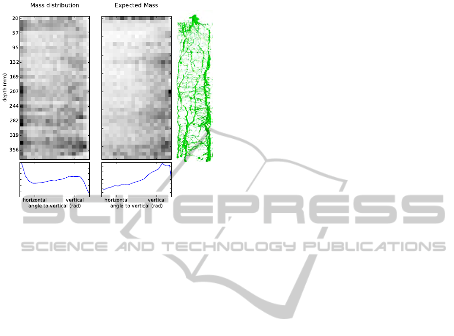
Distribution of Mass. The MRI voxel grid allows
to calculate the total mass of a plant. Using the model
constructed above, this mass distribution can now be
analyzed in new ways, which may be useful when
building statistical models of root growth. In Fig. 9,
we show the distribution of mass under the model (as
VISAPP 2012 - International Conference on Computer Vision Theory and Applications
30

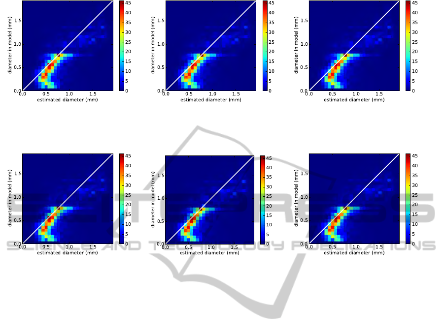
(a) (b) (c)
Figure 7: Histograms of true versus measured diameter at resolution 0.5 mm and ( a ) SNR 500, ( b ) SNR 150, and ( b ) SNR 50.
Diameter was measured using Eq. 2. For matching, each root was sampled in 0.2 mm steps and counted as “matched” if a
corresponding line segment in the other root was closer than one voxel size.
(a) (b) (c)
Figure 8: Same as Fig. 7, however with diameter estimated from local mass (cmp. end of Sec. 5).
derived in Sec. 5) as a function of the depth and the
root angle. We distinguish between expected mass of
a root at a certain depth/angle and the total mass at this
point. The data clearly shows that horizontal roots bind
most water (left), while vertical roots are less abundant,
but are expected to be heavier (middle). These results
agree with current biological understanding of the root
architecture of barley plants, which is characterized
by a small number of thick, vertically growing nodal
roots and a large number of fine horizontally growing
lateral roots, branching off the nodal roots.
6.4 Algorithm Runtime
On the 192 × 192 × 410 reference dataset, a complete,
partially parallelized run currently takes less than 20
minutes on a 12 × 2.67 GHz core Intel machine. For
the sake of algorithmic simplicity, the dataset currently
needs to provide cubic voxels. Thus, the coarse ver-
tical direction is upsampled resulting in a doubling
of the number of voxels. Avoiding this and using the
speed up potential through further parallelization of
the Hessian computation (across multiple computers)
and later steps (across multiple cores) may reduce the
computation time significantly.
7 SUMMARY AND
CONCLUSIONS
In this paper, we showed how to derive a structural
model of root systems from 3D MRI measurements
and assign mass and radius to found root segments.
From our experiments on the dependence of found
root length on image resolution and SNR, we conclude
that root system reconstruction strongly depends on
resolution, with better detection rates at higher reso-
lution. This is in coherence with the na
¨
ıve expecta-
tion. Also sensitivity to noise is as expected. SNR
below 100 severely effects detection accuracy of roots
with subvoxel diameters. Systematical errors of the
derived root structure occur at junctions, where branch-
ing angles are biased towards 90
◦
. A closer analysis
of junctions should therefore be investigated in future
research. However other measures are already well
applicable. Especially mass estimation (and radius
estimation when water density in roots is constant)
turned out to be robust against SNR reduction, while
geometry-based diameter estimates from Frangi scales
become less and less reliable. For healthy roots, ra-
dius from mass is an excellent alternative to geometry-
based measures, but in drying roots water density is
nonconstant and more sophisticated radius measure-
ments should be investigated.
3D RECONSTRUCTION OF PLANT ROOTS FROM MRI IMAGES
31

π/2 0 π/2 0
Figure 9: Mass distribution in root, w. r. t. depth and root
angle. Darker regions represent more mass. Left: Unnor-
malized mass, shows that horizontal roots are prevalent and
bind most of the water. Middle: Mass normalized by number
of roots, shows that vertical roots tend to have more mass
than horizontal ones. Directly beneath the soil surface, roots
tend to have more mass regardless of direction. Bottom plots
depict the marginal mass distribution of angle. Right: Model
visualization weighted by estimated mass (cmp. Fig. 3).
For real data of barley roots we showed, how the
derived structural and local quantities can readily be
used for plant root phenotyping.
REFERENCES
Armengaud, P., Zambaux, K., Hills, A., Sulpice, R., Pat-
tison, R. J., Blatt, M. R., and Amtmann, A. (2009).
Ez-rhizo: integrated software for the fast and accu-
rate measurement of root system architecture. Plant
Journal, 57(5):945–956.
Brown, J. M., Kramer, P. J., Cofer, G. P., and Johnson, G. A.
(1990). Use of nuclear-magnetic resonance microscopy
for noninvasive observations of root-soil water rela-
tions. Theoretical and Applied Climatology, pages
229–236.
Dijkstra, E. (1959). A note on two problems in connexion
with graphs. Numerische Mathematik, 1(1):269–271.
Dowdy, R., Smucker, A., Dolan, M., and Ferguson, J. (1998).
Automated image analyses for separating plant roots
from soil debris elutrated from soil cores. Plant and
Soil, 200:91–94.
Ferreira, S., Senning, M., Sonnewald, S., Keßling, P.-M.,
Goldstein, R., and Sonnewald, U. (2010). Comparative
transcriptome analysis coupled to x-ray ct reveals su-
crose supply and growth velocity as major determinants
of potato tuber starch biosynthesis. BMC Genomics.
Online journal, 11(17).
Frangi, A., Niessen, W., Vincken, K., and Viergever, M.
(1998). Multiscale vessel enhancement filtering. Medi-
cal Image Computing and Computer-Assisted Interven-
tation (MICCAI), pages 130–137.
Haacke, E., Brown, R., Thompson, M., and Venkatesan,
R. (1999). Magnetic Resonance Imaging, Physical
Principles and Sequence Design. John Wiley & Sons.
Haber-Pohlmeier, S., van Dusschoten, D., and Stapf, S.
(2009). Waterflow visualized by tracer transport in
root-soil-systems using MRI. In Geophysical Research
Abstracts, volume 11.
Jahnke, S., Menzel, M. I., van Dusschoten, D., Roeb, G. W.,
B
¨
uhler, J., Minwuyelet, S., Bl
¨
umler, P., Temperton,
V. M., Hombach, T., Streun, M., Beer, S., Khodaverdi,
M., Ziemons, K., Coenen, H. H., and Schurr, U. (2009).
Combined MRI-PET dissects dynamic changes in plant
structures and functions. Plant Journal, pages 634–
644.
Krissian, K., Malandain, G., Ayache, N., Vaillant, R., and
Trousset, Y. (1998). Model based multiscale detection
of 3d vessels. In Proceedings of the Workshop on
Biomedical Image Analysis, pages 202–210. IEEE.
Lindeberg, T. (1996). Edge detection and ridge detection
with automatic scale selection. In CVPR, pages 465–
470.
Lo, P., van Ginneken, B., and de Bruijne, M. (2010). Vessel
tree extraction using locally optimal paths. In Biomed-
ical Imaging: From Nano to Macro, pages 680–683.
M
¨
uhlich, M., Truhn, D., Nagel, K., Walter, A., Scharr, H.,
and Aach, T. (2008). Measuring plant root growth.
In Pattern Recognition 2008, volume 5096 of Lecture
Notes in Computer Science, pages 497–506. Springer.
Nagel, K. A., Schurr, U., and Walter, A. (2006). Dynamics
of root growth stimulation in nicotiana tabacum in
increasing light intensity. Plant Cell and Environment,
29(10):1936–1945.
Nakanishi, T., Okuni, Y., Furukawa, J., Tanoi, K., Yokota, H.,
Ikeue, N., Matsubayashi, M., Uchida, H., and Tsiji, A.
(2003). Water movement in a plant sample by neutron
beam analysis as well as positron emission tracer imag-
ing system. Journal of Radioanalytical and Nuclear
Chemistry, 255:149–153.
Pierret, A., Doussan, C., Garrigues, E., and Kirby, J. M.
(2003). Observing plant roots in their environment:
current imaging options and specific contribution of
two-dimensional approaches. Agronomy for Sustain-
able Development, 23(5–6):471–479.
Postma, J. A. and Lynch, J. P. (2011a). Root cortical
aerenchyma enhances the acquisition and utilization
of nitrogen, phosphorus, and potassium in zea mays l.
Plant Physiology, 156(3):1190–1201.
Postma, J. A. and Lynch, J. P. (2011b). Theoretical evidence
for the functional benefit of root cortical aerenchyma
in soils with low phosphorus availability. Annals of
Botany, 107(5):829–841.
Southon, T. E. and Jones, R. A. (1992). NMR imaging
of roots – methods for reducing the soil signal and
for obtaining a 3-dimensional description of the roots.
Physiologia Plantarum, pages 322–328.
VISAPP 2012 - International Conference on Computer Vision Theory and Applications
32

Tracy, S., Roberts, J., Black, C., McNeill, A., Davidson,
R., and Mooney, S. (2010). The X-factor: visualizing
undisturbed root architecture in soils using X-ray com-
puted tomography. Journal of Experimental Botany,
61(2):311–313.
van Rijsbergen, C. (1979). Information Retrieval. Butter-
worth, London, Boston, 2nd edition.
Waisel, Y., Eshel, A., and Kafkafi, U., editors (2002). Plant
Roots: The Hidden Half. Marcel Dekker, Inc.
3D RECONSTRUCTION OF PLANT ROOTS FROM MRI IMAGES
33