REAL-TIME LOCALIZATION OF OBJECTS IN TIME-OF-FLIGHT
DEPTH IMAGES
Ulrike Thomas
Institute for Robotics and Mechatronics, German Aerospace Center, 82234 Wessling, Germany
Keywords:
Object Localization, Pose Estimation, Time-of-Flight Sensors, Ransac.
Abstract:
In this paper a Random Sample Consensus (Ransac) based algorithm for object localization in time-of-flight
depth images is presented. In contrast to many other approaches for pose estimation, the algorithm does not
need an inertial guess of the object’s pose, despite it is able to find objects in real time. This is achieved by
hashing suitable object features in a pre-processing step. The approach is model based and only needs point
clouds of objects, which can either be provided by a CAD systems or acquired from prior taken measurements.
The implemented approach is not a simple Ransac approach, because the algorithm makes use of a more
progressive sampling strategy, hence the here presented algorithm is rather a Progressive Sampling Consensus
(Prosac) approach. As a consequence, the number of necessary iterations is reduced. The implementation has
been evaluated with a couple of exemplary scenarios as they occur in real robotic applications. On the one
hand, industrial parts are picked out of a bin and on the other hand every day objects are located on a table.
1 INTRODUCTION
Localization of known objects in images and acquired
scenes is of importance for many robotic applica-
tions, e.g. in assembly or service domains, where
robots have to interact autonomously with their en-
vironments. In this context, known objects need to
be located within a few seconds with such an accu-
racy in order to enable robots to manipulate these
objects. This problem is widely known as pose es-
timation in cluttered scenes, where objects might par-
tially be occluded. A robust and fast pose estima-
tion of known objects in such scenarios will support
robotic technologies to be brought into human envi-
ronments. Recently, time-of-flight sensors became
very popular and are used for some applications, e.g.
for pose estimation of the human body (Plagemann
et al., 2010), where real-time requirements have to be
met. In this paper, it is shown, how objects can be
localized in real-time in depth images acquired from
time-of-flight sensors. In the approach described in
this paper, no assumptions of inertial object poses are
required. The specific sensors applied for object lo-
calization in this paper are the Swissranger SR 4000
(Oggier et al., 2004) and the PMDs CamCube, pro-
viding intensity and depth images with a frame rate
of up to 50 Hz with a resolution of 174 × 144 and of
204 × 204 pixels, respectively. The calibration of the-
se sensorshas been described in (Fuchs and Hirzinger,
2008). Figure 1 illustrates intensity and depth images
acquired from given scenes by the time-of-flight sen-
sor. In this paper, only the depth images are used for
pose estimation. In general the localization problem
can be treated as a 6 dof pose estimation problem of
a rigid object; hence, the task is to estimate a pose
P := (R,
~
t) with R ∈ SO(3) and
~
t ∈ R
3
of a model in
the given depth image. The depth image is here con-
sidered as a point cloud P = {~p
1
,... ,~p
n
} with its sur-
face normals N = {~n
1
,. .. ,~n
n
} obtained from princi-
ple component analysis. The goal is to estimate poses
of objects in real time by extracting as much as possi-
ble a-priori model knowledge. This paper presents a
real-time object localization approach by using on the
one hand hash tables of features obtained from mod-
els and on the other hand by choosing a suitable sam-
pling strategy so that the Random Sample Consensus
(Ransac) algorithm is adapted to a more Progressive
Sampling Consensus (Prosac) approach. The content
of this paper is structured as follows: The next sec-
tion gives an overview about related work. The sec-
tion next after illustrates how the a-priori knowledge
of objects is extracted and processed, so that model
knowledge can be used efficiently for real-time pose
estimation. Section number four describes the main
part of the algorithm in particular the sampling strat-
egy and the hypotheses evaluation function. Section
Thomas U..
REAL-TIME LOCALIZATION OF OBJECTS IN TIME-OF-FLIGHT DEPTH IMAGES.
DOI: 10.5220/0003870707330737
In Proceedings of the International Conference on Computer Vision Theory and Applications (VISAPP-2012), pages 733-737
ISBN: 978-989-8565-03-7
Copyright
c
 2012 SCITEPRESS (Science and Technology Publications, Lda.)

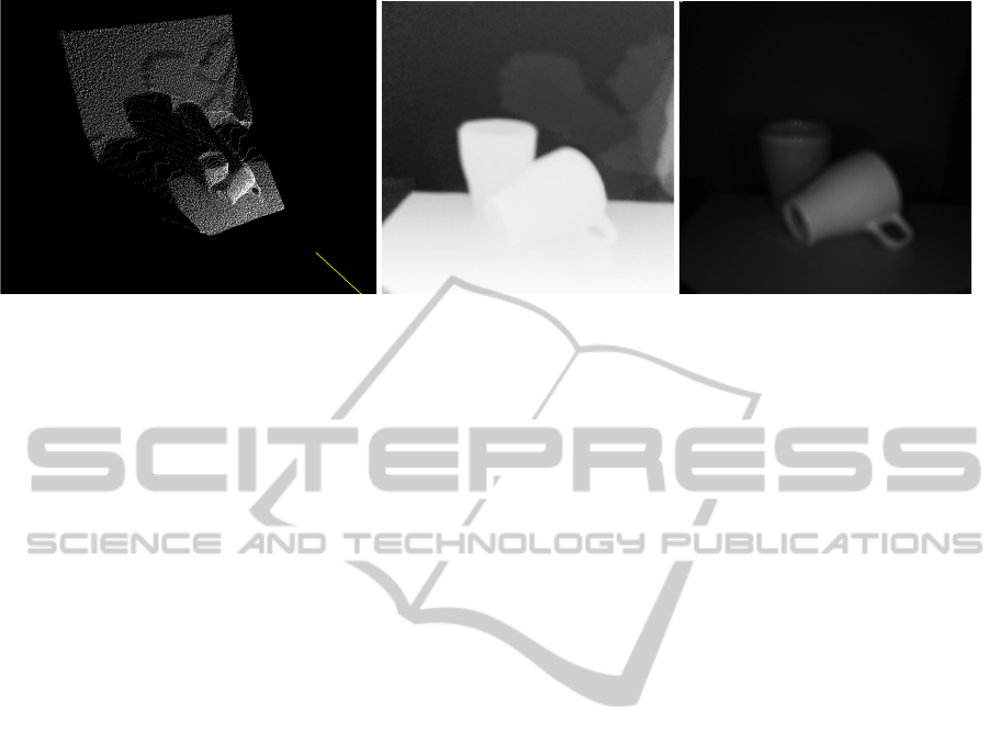
Figure 1: The algorithm is able to estimate object poses in uncluttered scenes. Illustrated a two cups arranged on a table. The
left image shows a 3d point cloud obtained from the depth image. The image in the middle shows the depth image itself and
on the right side the intensity image is depicted.
number five contains the evaluation part.
2 RELATED WORK
Ransac is well known for matching model data into
sensor data (Fischler and Bolles, 1981; Bolles and
Fischler, 1981). The original Ransac was illustrated
for fitting lines into 2D images. Since then, Ransac
has been applied to many applications. (Winkelbach
et al., 2004) show that it is possible to solve the 3d
puzzle problem using Ransac. As feature vector they
use surflet pairs, which are used in this paper, too.
(Buchholz et al., 2010) shows how the Ransac algo-
rithm can be applied to solve the bin picking prob-
lem using laser scanner data. (Schnabel et al., 2007)
apply Ransac for shape primitive detection in point
clouds. In order to estimate object poses in stereo
data obtained from image correlation (Hillenbrand,
2008) has provided an algorithm. For image regis-
tration and motion estimation (Nister, 2003) has ap-
plied the Ransac approach. In order to find certain
models in uncluttered point cloud scenes (Papazov
and Burschka, 2010) provide an algorithm, which
uses some different sampling strategies, which can
also be regarded as a Prosac approach. Prosac has
been successfully used for the registration of images
(Chum and Matas, 2005). Altogether, Ransac has be-
come very popular for pose estimation. All these ap-
proaches have in common, that they are not real-time
and mostly run for a few seconds on state-of-the-art
hardware to estimate positions of objects in unclut-
tered scenes. In contrast to most of the above men-
tioned algorithms, a progressive sampling strategy is
applied here, which takes the advantage of the model
based a-priori knowledge.
3 FEATURE EXTRACTION FROM
MODEL DATA
For generic object localization in real-time model
information needs to be processed prior to execu-
tion. In the past, most approaches required images
taken from the same sensor afflicted with same sen-
sor noise. In contrast, here, only point cloud data
of objects are applied as model data. These point
clouds might be obtained from images taken prior to
execution or from CAD-systems. Hence, model in-
formation is either available as triangle mesh – as a
simplest representation in CAD-systems – or as point
clouds. Hence, each object O
1
.. .O
m
can be mod-
eled by a set of vertexes O = {~v
1
,. ..~v
m
} with ~v
i
∈ R
3
and their corresponding surface normals. The surface
normals are estimated by means of principle com-
ponent analysis on at least five up to eight closest
neighbors N := {~n
i
,. .. ,~n
m
} with ~n
i
∈ R
3
. This kind
of model generation is indeed very generic and de-
pends not on a certain set of data. Figure 2 illustrates
the original model data and the features drawn from
theses models. Remember, the original Ransac al-
gorithm takes two points ~p
i
, ~p
j
from the input data
set P = {~p
1
,. .. ,~p
n
}, and searches for the same two
points ~v
i
, ,~v
j
in the model data set V = {~v
1
,. .. ,~v
m
}.
Figure 2 illustrates a selected tuple (~p
i
,~p
j
). Each
point is assumed to be an oriented point with respec-
tive point normals ~n
i
,~n
j
. It is shown how these fea-
ture pairs can be used to align the objects. For real-
time object localization it is very important to access
theses features in near O(1) time complexity, scince
the algorithm takes iteratively such features from the
acquired data set and seeks for the corresponding fea-
tures in the model set. Hence, a hash table suites well
to provide efficient access to model features. The hash

Figure 2: The model features, which are inserted into the
hash map. For each pair of points the feature vector is de-
termined and hashed, if the distance of points is not closer
than a given threshold.
function must be as unambiguous as possible. Hence,
given two vertexes (~v
i
,~v
j
) with their vertex normals
(~n
i
,~n
j
) from the model data the feature vector f ∈ R
4
is defined by:
f (v
i
,v
j
) :=





||~v
i
−~v
j
||
∠(~n
i
,~v
j
−~v
i
)
∠(~n
j
,~v
i
−~v
j
)
atan2(
~n
i
·(
~
d
i j
×~n
j
)
(~n
i
×
~
d
i j
)·(
~
d
i j
×~n
j
)
)





(1)
with
~
d
i j
= ~v
i
−~v
j
. This feature vector has four di-
mensions. Hence a hash table of size N
4
is applied
and N need to be adjusted to the available storage
size. For this hash function the angular values be-
tween [0,...,2π] are mapped to the range [0,. ..,N].
For the translational parameter of f , the bounds b
min
and b
max
are chosen according to the model data.
b
max
= max{||~v
i
−~v
j
|| |∀~v
i
,~v
j
∈ O ∧ i 6= j}
b
min
= b
max
· 0.33
(2)
Therewith, the range of the hash table is adopted to
values between the maximum possible translational
distance of two point pairs and the minimum distance,
which is bounded by one third of the maximum dis-
tance. It has been shown in experiments, that this
choice is a reasonable bound. The explanation reads
as follows: The smaller the range is for a feature
the better are the matches of a point pair in the hash
table and consequently the algorithm is able to find
good matches much faster. Additionally to adjust-
ing the hash map size to sizes of objects, the bounds
are applied to enforce the algorithm to draw sam-
ples, which correspond more likely to the same ob-
ject. Thereby, the random sampling consensus strat-
egy turns more into a progressive sampling strategy,
which is explained in more detail in the next section.
Note, that here for each object a separate hash table is
used, which is much faster than using only one hash
table, because the size of the hash table can be fitted
better to the size of the objects. Due to the time con-
suming filling of the hash table, this is processed in an
off-line phase.
4 RANSAC FOR OBJECT
LOCALIZATION
Ransac is known very well for model fitting into
measured data sets. In general the algorithm draws
two samples randomly out of the data sets and seeks
for the corresponding feature pair in the model data.
Therewith, an object hypothesis is generated and eval-
uated. For the sampling strategy we have applied a
progressive approach, for which we can show that the
number of iterations is reduced to find certain objects
in a scene. Additionally, an efficient evaluation func-
tion is implemented able to estimate the quality of hy-
potheses very accurately. Therewith our approach can
be executed in real-time. In general, the steps of the
algorithms can be described as follows:
1. For each object o
i
a hash table has to be generated
which is filled by feature vectors obtained for each
tuple (~v
i
,~v
j
) of oriented point pairs as mentioned
above.
2. Start sampling by drawing the first point ~p
i
from
the measured data set P = {~p
i
.. .~p
n
} at random
3. Sampling the second point ~p
j
by applying a ball
of radius r with the first sample point as center
point. The radius is assigned with the bounds of
the object for which the pose should be estimated.
Given n objects to be found in a scene, we approx-
imate r as upper bound over all searched objects
with max
b
max
∀O
.
4. Regarding to the chosen pair of point (~p
i
,~p
j
) de-
termine the feature vector f (~p
i
,~p
j
) and look it up
in the hash table with the corresponding key. Let
H be the set of hypotheses found in in the hash
table for the chosen feature pairs f (~v
i
,~v
j
), then
determine for each hypothesis h
i
∈ H the aligned
transformation for rigid motion R ∈ SO(3) and
t ∈ R
3
, see Figure 2
5. Evaluate the hypothesis. If it is a suitable hypoth-
esis a confidence value is returned.
6. As long as no good hypotheses for the object is
found and the time bound is not reached continue
with step 2.

4.1 Progressive Sample Consensus
With the progressive sampling strategy it can be
shown that the number of necessary iteration can be
reduced. Given a data set of measured range image
with N points, and assuming in the data set an ob-
ject which is modeled by m points, the probability of
finding the object is provided as follows. Note, that
the number of inliers is set to m where the number of
outliers is set to N. The probability p of finding two
inliers in a single path is given approximately by the
ratio of:

m
2

/

N
2

≈

m
N

2
(3)
The choice of points is assumed to be independent,
because neglecting the points already drawn reduces
the expensive deletion of points in hierarchical data
sets. Now, let k be the number of iterations, where
no two inliers have been chosen. Then we can assign
the probability that Ransac has not converged against
a solution after k iterations by:
1 − p(o,k) = (1 −

m
N

2
)
k
(4)
it follows that the number of iteration k necessary to
find two inliers is given by the ratio:
k =
log(1 − p(o,k))
log(1 −

m
N

2
)
(5)
Assuming the ratio between inliers and outliers is set
to 10% and a probability of 50% is expected to fit the
model data into the data set, the number of iterations
necessary to be executed is given by 68. If we want
to reduce the necessary iterations, we might draw the
second point out of a ball of size r which contains R
outliers with R  N. The probability of choosing a
ball with only R outliers might be given by the ratio
of (m/R) with 20% inliers at average. Then, the prob-
ability of drawing two inliers after k iterations can be
estimated by:
p(o,k) = 1 − (1 − (

m
N

·

m
R

)
k
) (6)
and hence due to the ratio of 20% the number of it-
erations is reduced to 34, which is the half. But this
holds only if R and respectively the ball size r is cho-
sen in an appropriate way. It is realized by applying
a ball search in the here used kd-tree data structure.
The ball size is set to the upper bounds of the model
data set.
4.2 Aligning Two Hypotheses
If a suitable hypothesis is found in the hash table, the
model data has to be aligned to the drawn data. Given
the feature vector found in the hash table f (~v
i
,~v
j
)
with its corresponding point normals (~n
v
i
,~n
v
j
) and the
feature vector obtained from drawing two samples
f (~p
i
,~p
j
) respectively with its normals (~n
p
i
,~n
p
j
) the
rigid body transformation can be determined in the
following way. First we aligning the translational vec-
tor
~
t
∆
by:
~
t
∆
=
1
2
(~v
j
+~v
i
−~p
j
+~p
i
) (7)
and for the rotational part, we align the normal vectors
and obtain the rotation matrix Rot ∈ R
3×3
Rot
W
Feat
B
:=

(~v
j
−~v
i
)·(~v
j
−~v
i
)
||(~v
j
−~v
i
)×(~v
j
−~v
i
)||
(~x·~n
v
i
)
||~x×~n
v
i
||
(~x·~y)
||~x×~y||

(8)
and respectively the rotation matrix for the features
taken from model data Rot
W
Feat
A
. The obtained trans-
formation applied to the model data ~v
i
is then given
by Rot
W
Feat
A
·(Rot
W
Feat
B
)
−1
~v
i
+
~
t
∆
. Therewith we get hy-
potheses from drawing point pairs out of the measured
data set which have to be evaluated.
4.3 Evaluating Hypotheses
The evaluation function has to be efficient and accu-
rate, which means that no good hypotheses should be
overlooked and that many hypothesis can be evaluated
in a reasonable amount of time. For these objectives
we define a model point ~v
i
with its point normal ~n
transformed to ~v
0
i
by the above given rigid transfor-
mation. A model point is defined to be in contact
with a measured data point ~p
j
, if their distances are
smaller then a given threshold δ and the normal vec-
tors directs toward the camera coordinate system. The
distance can be estimated very fast using hierarchical
data structures like kd-trees. The hypothesis error is
hence given by following equation:
1
c
2
contact
s
∑
∀~v
0
i
∈ O
g(~v
0
i
) (9)
The distance function g is denoted by:
g(v
i
) :=



d = min
∀p
j
{|| v
i
− p
j
||} if d ≤ δ and
~v
i
visible
δ else
(10)
With this evaluation function, those hypotheses are
assigned with lower cost, whose number of contact
points is higher.
5 EVALUATION
The evaluation of the algorithm has been carried out
by using some different objects. For each object the

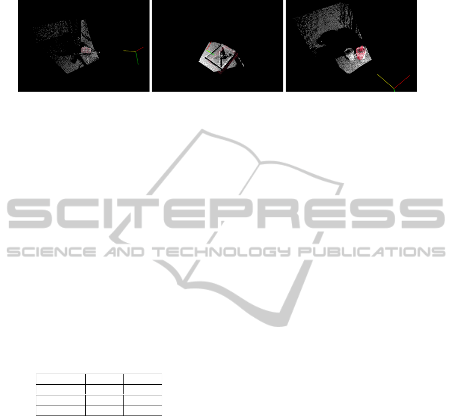
Figure 3: Results for object localization. Left: Finding a box modeled by 625 points has been located. Note, that many
symmetries are in the depth image, which makes it much more difficult to find an accurate solution. Middle: For solving the
bin picking problem; the bin has been located. Right: Two cups are arranged; the better solution is chosen as it can be seen.
appropriate hash table is filled as described in sec-
tion three. For evaluating the pose estimation ap-
proach, the algorithm has been repeated 20 times and
the mean execution time is depicted in Table 1. Ad-
ditionally, to the original Ransac approach the Prosac
based sampling strategy has been applied. The Figure
3 illustrates the results. It is shown that object poses
can be estimated very fast with a reasonable position
and rotation error. The output generated by our ap-
proach should be used as an inertial solution for ei-
ther the ICP (iterative closed point) algorithm or the
Kalman filter, if real-time requirement must be met.
The computation times of both Ransac and Prosac are
listed and it can be shown that the Prosac approach
converges much faster against a reasonable solution.
Table 1: Evaluation time for scenarios illustrated in Figure
3. The computation has been carried out on an Intel Xeon
2,7 GHz CPU with 3 GB Memory.
Scenarios Ransac Prosac
example 1 82 ms 49 ms
example 2 748 ms 498 ms
example 3 831ms 501 ms
6 CONCLUSIONS
For object localization a Ransac algorithm has been
implemented and is compared to a Prosac approach.
With the Prosac approach the number of iterations to
find two inliers is reduced. Thereby an algorithm has
been provided which can be applied in real-time for
pose estimation. We suggest to use it as an inertial
pose guess for a particle filter or a Kalman filter. The
approach can be adopted to any depth images or point
clouds. The presented method will be applied to un-
cluttered scenes represented as point clouds as well
as depth images obtained from stereo vision. Fur-
ther on it is planned to compare this approach with
the fast point feature histograms registration method
described in (Rusu et al., 2009).
REFERENCES
Bolles, R. and Fischler, M. A. (1981). A ransac-based ap-
proach to model fitting and its application to finding
cylinders in range data. In Proc. IJCAI, pages 637–
643.
Buchholz, D., Winkelbach, S., and Wahl, F. M. (2010).
Ransam for industrial bin-picking. In ISR/Robotics
2010, pages 1317–1322.
Chum, O. and Matas, J. (2005). Matching with prosac -
progressive sampling consensus. In Proc. Conf. Com-
puter Vision and Pattern Recognition.
Fischler, M. and Bolles, R. (1981). Random sample consen-
sus: A paradigm for model fitting with applications to
image analy- sis and automated cartography. CACM,
24(6):381–395.
Fuchs, S. and Hirzinger, G. (2008). Extrinsic and depth
calibration of tof-cameras. In Proc. Conf. Computer
Vision and Pattern Recognition.
Hillenbrand, U. (2008). Pose clustering from stereo data.
In VISAPP International Workshop on Robotic Per-
ception, pages 23–32.
Nister, D. (2003). Preemptive ransac for live structure and
motion estimation. In ICCV, pages 199–206.
Oggier, T., Lehmann, M., and R. Kaufmann, M. Schweizer,
M. R. (2004). An all-solid-state optical range camera
for 3d real-time imaging with sub-centimeter depth
resolution(swissranger). In Proc. SPIE, volume 5249,
pages 534–545.
Papazov, C. and Burschka, D. (2010). An efficient
ransac for 3d object recognition in noisy and occluded
scenes. In ICCV.
Plagemann, C., Ganapathi, V., Koller, D., and Thrun, S.
(2010). Real-time identification and localization of
body parts from depth image. In Proc. International
Conference on Robotics and Automation.
Rusu, R. B., Blodow, N., and Beetz, M. (2009). Fast point
feature histograms (fpfh) for 3d registration. In ICRA.
Schnabel, R., Wahl, R., and Klein, R. (2007). Efficient
ransac for point-cloud shape detection. In Eurograph-
ics, pages 1–12.
Winkelbach, S., Rilk, M., Schoenfelder, C., and Wahl, F.
(2004). Fast random sample matching of 3d frag-
ments. In PatternRecognition (DAGM 2004), Lecture
Notes in Computer Science 3175, pages 129–136.