
PREDICTION MODEL OF INPATIENT MORTALITY FOR
PATIENTS WITH MYOCARDIAL INFARCTION
Hynek Kružík
1
, Jiří Vomlel
2
, Václav Kratochvíl
2
, Petr Tůma
1
and Petr Somol
2
1
GNOMON Healthcare Solutions s.r.o., Faltysova 1500/18, Prague, Czech Republic
2
Institute of Information Theory and Automation, Academy of Science of the Czech Republic, Prague, Czech Republic
Keywords: Data mining, Machine learning, Artificial intelligence, Logistic regression, Predictive model, Acute
myocardial infarction.
Abstract: We propose and investigate a prediction model of inpatient mortality for patients with myocardial
infarction. The model is based on complex clinical data from a hospital information system used in the
Czech Republic. The prediction of the outcome is an important risk-adjustment factor for objective
measurement of the quality of healthcare; thus it is a very important factor in healthcare quality assessment.
For our experiments we studied hospital mortality in acute myocardial infarction, because: (1) this indicator
is reliably detectable from available data; (2) treatment of acute myocardial infarction has a significant
socio-economic impact; and (3) the prediction of mortality based on admission findings is the subject of
many research papers and thus, we have a good benchmark for our experimental results. We considered
only variables that convey information about the patient at the time of admission. We selected 21 out of 637
variables and used them as predictors in logistic regression to form a prediction model for hospital
mortality. The achieved prediction accuracy was 85% and the size of the area under the ROC curve was
0.802. The results are based on a relatively small data sample of 486 patient records. Our future work will
aim at increasing the accuracy by using a larger data set.
1 INTRODUCTION
The results of medical treatment depend not only on
appropriate selection and proper execution of the
treatment, but also on initial individual conditions of
the patient. Evaluation of the patient’s initial
conditions is applicable in two major tasks: (1) in
estimating the prognosis of the patient in order to
select the most efficient treatment, e.g., the selection
of an adequate mix of interventions and medications,
or to decide on timely referral to the facility with
higher or (less commonly) lower specialization, i.e.,
for risk stratification, (2) for the retrospective
statistical evaluation of the care using standardized
quality indicators, i.e., for the risk adjustment task.
Conceptually, these two processes must be
mutually consistent. Risk adjustment of the outcome
quality indicators is essentially based on the
stratification of the risks and on empirical
knowledge and scientific evidence of the influence
which each patient's individual risk factors have on
the result of care in the group of patients.
In practice, there are significant differences in
performing risk stratification and risk adjustment
(standardization). Risk stratification is done in real
time by physicians and it is based on all available
information while standardization of the risks is
done retrospectively, mostly by medical or
regulatory authorities. During risk stratification of a
particular patient, all relevant information is
available or can be relatively easily obtained from
the clinical documentation or from additional
medical investigation. Retrospective evaluation of
the quality of outcomes is subject to many
restrictions: e.g., missing values of the variables
cannot be completed; evaluation is mostly done
outside of the healthcare facility and is based on
limited sets of available data which have not
necessarily been designed for the purpose of quality
measurement. These data sets are in general denoted
as “administrative” and the models based on them
are generally called “administrative” models.
Administrative data, i.e., demographic data,
diagnoses, procedure codes, and coded results of
hospitalization case outcomes are part of an inpatient
service reimbursement form which is utilized for all
inpatient cases reimbursed from the mandatory
453
Kružík H., Vomlel J., Kratochvíl V., T˚uma P. and Somol P..
PREDICTION MODEL OF INPATIENT MORTALITY FOR PATIENTS WITH MYOCARDIAL INFARCTION.
DOI: 10.5220/0003873504530458
In Proceedings of the International Conference on Health Informatics (HEALTHINF-2012), pages 453-458
ISBN: 978-989-8425-88-1
Copyright
c
2012 SCITEPRESS (Science and Technology Publications, Lda.)

healthcare insurance scheme in the Czech Republic.
Differentiation of positive or negative results as
they relate to quality of service is crucial for
efficient allocation of funds; as such it is (or should
be) of primary interest to the insurance companies.
In order to create and validate an administrative
prediction model, a clinical model, i.e., risk-adjusted
clinical model, should be built first as a “gold
standard”.
For our experiments with risk-adjusted clinical
models we chose hospital mortality in acute
myocardial infarction, because: (1) this indicator is
reliably detectable from available data; (2) treatment
of acute myocardial infarction has a significant
socio-economic impact; (3) prediction of mortality
based on admission findings is the subject of many
research papers, thus we have a good benchmark for
our experimental results; and (4) no outcome-
prediction models are currently used in the Czech
Republic; thus they are a necessary novelty in
quality measurement.
Our work has been motivated by the work
published at the Yale University (Krumholz, H. M.,
et al, 2007).
2 METHODS
2.1 Risk Adjustment
Risk adjustment is a statistical process used to
identify and adjust for variations in patient outcomes
that stem from differences in patient characteristics
(or risk factors) across healthcare organizations in
order to achieve better comparison of patient
outcomes between different organizations and to
improve the interpretability of results. The quality of
healthcare can be measured by several types of
indicators: by mortality, by re-hospitalization rate or
by complication rate. In this part, we will show
reasons and principles of risk adjustment of a
mortality indicator. Standardization of other types of
indicators follows the same principles.
A straightforward comparison of mortality rate
of two different healthcare facilities will not give
objective results as it also depends on the presence
of risk factors at the time of health care encounters.
Patients may experience different outcomes
regardless of the quality of care provided by the
healthcare organization, so comparing patient
outcomes across healthcare organizations without an
appropriate risk adjustment could be misleading. By
adjusting for the risks associated with outcomes of
interest, risk adjustment facilitates a fairer and more
accurate inter-organizational comparison. (CMS,
2005).
There are two essential methods: (1) case
stratification, i.e., decomposition of cases into more
homogeneous sub-groups based, for example, on age
and/or sex grouping, or (2) standardization of results
(indicators), i.e., risk-adjustment. The first method,
however, is disadvantageous both in terms of
statistics (subgroups will often have small numbers
of patients) and in terms of subsequent interpretation
(different subgroups may have different comparative
results and it may not be clear how the provider
should actually be evaluated with respect to the
overall quality in the clinical area).
2.2 Selection of Risk Factors
The requirements for the selection of risk factors
applicable in the standardization process indicators
are as follows: (i) there must be a statistically
significant relationship between risk factor and the
outcome indicator. For example, if the probability of
death from myocardial infarction is related to the
value of blood pressure at the time of admission,
then it is included as a risk factor. The prediction
model should also reflect situations in which certain
combinations of factors have greater impact than
each of the individual factors alone; (ii) the
composition of patients, in terms of risk factors,
must be different in different healthcare facilities.
Otherwise, there is no need to carry out
standardization, although there is a strong
correlation between the indicator and risk factor – all
healthcare facilities are "disadvantaged" in the same
way. In practice, this requirement is usually met, as
healthcare facilities usually have different
distributions of risk factors among their patients; (iii)
each risk factor must clearly reflect the condition of
the patient upon admission to a healthcare facility
and may not be the result of the treatment process
itself; (iv) each risk factor has to be reliably
documented within the available data –
unfortunately, this is a very limiting restriction in
many cases, and especially in administrative data.
It is obvious that the correction of the
measurement bias is never perfect. Even after
standardization, residual bias remains. Residual
distortion can, for example, be caused by risk factors
that are not yet known or that are not reflected in the
data.
2.3 Standardization of Indicators
When standardizing the quality indicators it is first
HEALTHINF 2012 - International Conference on Health Informatics
454

necessary to find and express the relationship
between the indicator and each risk factor. Suppose
that the risk factor is age and the outcome indicator
is the hospital mortality of acute myocardial
infarction. Based on data from the entire set of
healthcare facilities (standard population) it is
therefore necessary to express, with the help of
statistical methods, the relationship between the
patient's age and the likelihood of death from heart
attack. Then, for each hospital the correlation index
(CI) is calculated. CI is defined as the proportion of
two variables: the actual number of deaths and the
predicted (expected) deaths: CI = the actual number
of deaths / predicted (expected) number of deaths.
The expected number of deaths in a hospital is
the sum of individual probabilities of death of all
patients admitted to the hospital, determined with
respect to their risk factors. The expected number of
deaths is the number of deaths that would be
expected if the hospital held the same mortality risk
as the population of all hospitals. If the actual
number of deaths differs from the expected number,
we can conclude there are internal factors that have
an influence on the number of deaths in this
particular hospital. The correlation index is a
dimensionless number that indicates the relative
position of the hospital compared with the average:
an index value greater than one indicates above
average mortality, while an index value less than one
indicates the contrary, i.e., below average mortality.
Standardized mortality rate is obtained by
multiplying the index value by general mortality,
i.e., the average mortality for all hospitals:
standardized mortality = general mortality * CI.
The result of standardization of the indicator is
the value of the indicator on the condition that the
hospital had the same distribution of risk factors as
the entire group of providers.
2.4 Patient Sample
Our initial study is comprised of cases from one
Czech hospital. After exclusion of patients
transferred for treatment elsewhere, we selected all
patients admitted to the hospital with the main
diagnosis of acute myocardial infarction (ICD-10
codes in the range of I210 - I214). Our resulting data
set consisted of 486 patients (both male and female,
without age restrictions). The data set includes the
usual demographic and administrative data including
outcome status, principle and secondary diagnoses
coded using ICD-10, list of procedures coded using
the Czech national list of medical procedures, and
laboratory results. In addition, we had complete
information about previous hospitalizations in the
same hospital during the 12 months prior to the
respective hospitalization. In total we considered
637 variables (possible risk factors). Only 151
patient records included all values of the potential
risk factors. Patient records with missing values
were not excluded; instead, to keep maximum usable
information, we used a method of imputation of
missing data values (Rubin, D. B., 1987).
2.5 Statistical Analysis
The first and most difficult step in the
standardization of a selected indicator is to identify
relevant risk factors and formally characterize their
influence on the selected indicator. Often (see, e.g.,
Krumholz et al, 2007) the relationship between the
risk factors and the selected indicator is expressed
using logistic regression.
Let P(Y = 1|X=x) denotes the probability that the
variable Y reaches the value 1 given the value x of
the vector of risk factors X. In our case it is the
probability that the patient will die within 30 days
after admission to the hospital.
The logistic regression model defines the
relationship between the dependent variable and a
vector of the risk factors having values of
vector . The relationship is defined by the logistic
function
P
(
Y
=1|=
)
=
exp
(
′
)
1+exp
(
′
)
,
(1)
where is the vector of parameters to be found and
′
denotes its transposition. Vector is usually of
the form
(
1,
)
and the first component of vector ,
referred to as
, is the absolute member (intercept).
First, we selected candidates for the risk factors
based on the information gain method. Information
gain of each risk factor and the dependent variable
is defined as
(
,
)
=
(
)
+
(
)
− (,) ,
(2)
where
(
)
is the entropy of variable defined as
(
)
=−(=)log(=)
(3)
and (,) is the mutual entropy of variables and
defined similarly as
(
,
)
=−
(
=,=
)
,
log
(
=,=
)
.
(4)
Log is the binary logarithm. The higher the
information gain, the more information variable
PREDICTION MODEL OF INPATIENT MORTALITY FOR PATIENTS WITH MYOCARDIAL INFARCTION
455

brings about the value of variable . Absolute values
of laboratory tests have been used, not relative
values against the standard range for age and sex of
the patient. Values of continuous variables were
divided into ten bins for the purpose of information
gain calculations. For further processing, we ranked
only variables whose information gain was greater
than 0.01. The finally selected variables are given in
Table 1.
Table 1: Variables with an information gain greater than
0.01.
Code Description Information
gain
Urea Serum urea 0.11674202
Crea Serum creatinine 0.09532763
Leuco Leukocytes in full blood 0.06820710
I48 Atrial fibrillation and flutter 0.02425088
O.E78 Disorders of lipoprotein
metabolism and other
lipidaemias
0.02318073
O.I20 Angina pectoris 0.02044021
O.I48 Atrial fibrillation and flutter 0.01997538
I73 Other peripheral vascular
diseases
0.01971532
O.I27 Other pulmonary heart
diseases
0.01971532
O.I73 Other peripheral vascular
diseases
0.01971532
Age Patient’s age 0.01926587
O.I46 Cardiac arrest 0.01851840
K92 Other diseases of digestive
system
0.01758336
O.I21.0 Acute transmural myocardial
infarction of anterior wall
0.01651995
I74 Arterial embolism and
thrombosis
0.01576957
I42 Cardiomyopathy 0.01474711
O.I42 Cardiomyopathy 0.01474711
O.I10 Essential (primary)
hypertension
0.01471863
O.I21.1 Acute transmural myocardial
infarction of inferior wall
0.01440448
O.I64 Stroke, not specified as
haemorrhage or infarction
0.01358037
I27 Other pulmonary heart
diseases
0.01349612
K29 Gastritis and duodenitis 0.01338366
K62 Other diseases of anus and
rectum
0.01290232
L95 Vasculitis limited to skin, not
elsewhere classified
0.01290232
K57 Diverticular disease of
intestine
0.01217010
I50 Heart failure 0.01158408
O.I21.4 Acute subendocardial
myocardial infarction
0.01140944
K80 Cholelithiasis 0.01054740
Variables prefixed with "O" indicate diagnoses
that the patient encountered during the examined
hospitalization. Other diagnoses (without the "O"
prefix) were taken from the patient's hospitalizations
within one year prior to the hospitalization studied.
Variables in Table 1 were then used for training
the logistic regression model. For this purpose the
values of all the considered variables were
normalized to the interval <0, 1>. Some patients did
not have all selected variables examined. One option
for such patients was their exclusion from the data
set. This would, however, significantly reduce the
available data. Therefore, we chose Multivariate
Imputations by Chained Equations (cf. Rubin, D. B.,
1987 or Buuren, S., at al, 2006) to substitute the
missing values. Alternatively, we also tested the
replacement of missing risk factor values by the
average value of this factor, but in this case the
results proved to be less accurate. We also excluded
variables that were causing singularities: O.I73,
O.I42 and L95, and also those that might yield
misleading information due to co-morbidities: O.I20,
O.I48, O.I46 and O. I64.
For the actual learning of the model parameters
of logistic regression we have used the glm module,
which is part of the statistical system R (R
Development Core Team, 2010).
3 RESULTS
The resulting model is described in Table 2. The
first column includes the names of the risk factors as
in Table 1.
In the second column there are individual
coefficients , i.e., the components of vector of
the logistic regression formula. Standard deviations
of the coefficient are in the third column, and the
fourth column contains the corresponding values of
Student's t-test -- i.e., whether coefficient has the
given mean value. The fifth column shows the
number of degrees of freedom of the Student's t-
distribution calculated in accordance with (Barnard
and Rubin, 1999). The last column gives the
probability of alternative hypotheses of the t-test
presented. Values lower than 0.05, which
corresponds to the static level of significance of 5%,
are shown in bold. These values indicate that the
hypothesis that coefficient β has the given value as
its mean value is accepted at a static level of
significance of 5%.
The values of coefficients β thus can be roughly
interpreted as follows: the greater a positive number,
the greater the influence of the corresponding risk
factor on the probability of death. The lower a
negative number, the greater the influence of the
corresponding risk factor on the probability of
HEALTHINF 2012 - International Conference on Health Informatics
456

Table 2: Parameters of the logistic regression model.
Code
SD t value degrees of
freedom
Alt. hyp.
(Intercept) -2.1060975 1.2651842 -1.664656859 31.598080 0.105868127
Urea
8.6381220 3.2418691 2.664549922 6.539030 0.034363798
Crea -1.0298399 3.1864171 -0.323196842 6.948143 0.756055460
Leuco 1.3401639 2.5917890 0.517080649 6.072126 0.623388122
I48
1.1774437 0.5043932 2.334376623 62.932775 0.022781215
O.E78
-1.1969985 0.4437995 -2.697160631 456.217585 0.007252314
I73 24.2072289 3127.7478688 0.007739508 463.999987 0.993828154
O.I27 22.4904111 3055.1132840 0.007361564 463.999942 0.994129539
Age -0.8665293 1.2988153 -0.667169004 46.748401 0.507944173
K92 0.1754608 2.1248919 0.082573969 260.797168 0.934253641
O.I21.0 2.0831447 1.2175409 1.710944339 14.713859 0.108083943
I74 0.8435731 1.2306952 0.685444349 363.623078 0.493500307
I42 18.6880782 3580.0597075 0.005220047 463.999856 0.995837268
O.I10
-1.7197621 0.5011027 -3.431955378 32.644378 0.001645515
O.I21.1 -18.4366694 1142.1321492 -0.016142326 463.999889 0.987127785
I27 -0.3723272 2.1099515 -0.176462425 220.553439 0.860092594
K29 -0.6493484 1.1797607 -0.550406839 49.675659 0.584507085
K62 1.6111716 3.1727303 0.507818643 83.887081 0.612913195
K57 1.5036105 1.8285737 0.822285931 17.330469 0.422084093
I50 -0.2095659 0.5698730 -0.367741513 18.221241 0.717302894
O.I21.4 -0.2596627 1.1148068 -0.232921682 9.406510 0.820811800
K80
1.4525334 0.5681741 2.556493236 388.428873 0.010952816
survival. The number in the last column tells us to
what extent this effect is statistically significant. For
values greater than 0.05 (which is true for most of
our risk factors), we can say that the impact on the
probability of death was not statistically proven in
our data set. However, it is necessary to remark that
these results are affected by the small number of
patients in our data set.
3.1 Evaluation of Results of the
Logistic Model
For a reliable evaluation of the quality of the trained
prediction model, independent data that were not
used to learn the model are needed. For this purpose
we used the method of K-fold cross-validation,
where K had a value of ten. We randomly divided
the data set into ten groups of approximately equal
size. The remaining nine groups were used to train
the model which was then validated on the selected
group. This procedure was repeated for each of the
ten groups. The results presented below summarize
all partial results.
The basis for evaluation is the confusion matrix,
which includes numbers of true positive (tp) and
false positive (fp) predictions that the patient will die
and true negative (tn) and false negative (fn)
predictions that the patient will not die.
The results of our model were as follows: tp =
28, tn = 383, fp = 9, fn = 66. Based on these values
we can express the results of model evaluation:
accuracy = 0.85, precision = 0.76, recall =
0.30, and false alarm rate = 0.02.
The output of the logistic regression model is not
only an estimate of whether or not the patient dies
within 30 days, but it gives the probability with
which this event occurs. Also, it is possible to
change the decision threshold (which is normally set
to 0.5) of the classification. This enables us, for
example, to increase recall at the expense of
precision and vice versa. The overall behavior of
such a classifier is best characterized by the ROC
curve, see Figure 1.
The ROC curve shows the dependence of recall
and false alarm rate on the value of the threshold
(threshold values are shown below the curve in
Figure 1). The higher the curve is located, the better
results the model gives. A good measure of
classifier’s performance is the size of the area under
the curve, i.e., the ROC area. The maximum value
that represents the ideal classifier is 1.0. On the
contrary, a value of 0.5 can be reached by a random
classifier. The value of the ROC area of our model
was 0.802.
PREDICTION MODEL OF INPATIENT MORTALITY FOR PATIENTS WITH MYOCARDIAL INFARCTION
457
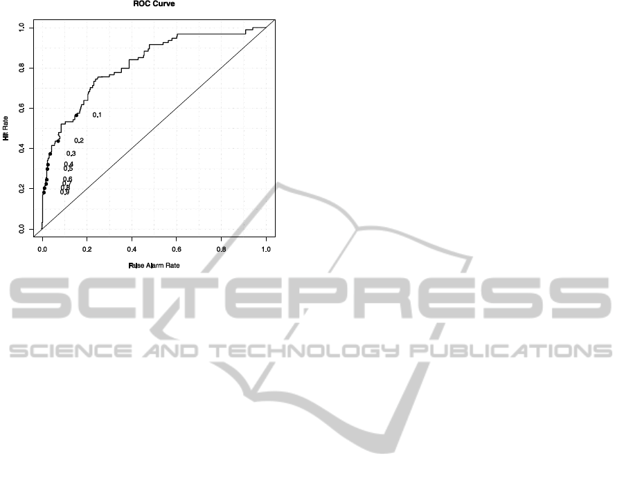
Figure 1: ROC curve of the classifier.
4 CONCLUSIONS
In this work we studied the standardization of
outcome indicator “hospital mortality in acute
myocardial infarction.” Although we had a relatively
small data sample and we used only the main and
secondary diagnoses and the results of three
laboratory tests to build a predictive model, we
succeeded in predicting the 30-day mortality of
patients relatively successfully. The achieved
accuracy was 85% and the size of the area under the
ROC curve was 0.802. With regard to the statistical
properties of predictive models of this type, it can be
expected that a better prediction could be achieved
by using other data from an electronic patient record,
such as ECG, localization of pain and blood pressure
(these data are stored only in free text format and
would involve difficult pre-processing to enable us
to use them in the classifier construction; this was
beyond the scope of this paper). For practical use of
our result in the standardization of mortality
indicators, it will be necessary to train the model
using a larger data set from many hospitals. Then it
will also be possible to make a better medical
interpretation of the achieved results.
Another challenge, which we intend to address in
the future, is researching the effect of a combination
of several risk factors and the use of ratings of
laboratory test results performed with respect to the
normal ranges for a particular sex and age
combination, rather than with respect to their
nominal values only.
ACKNOWLEDGEMENTS
This work was carried out under the grant of the
Ministry of Education of the Czech Republic No.
2C06019, ZIMOLEZ.
REFERENCES
CMS, 2005. Specification Manual for National Hospital
Quality Measures, version 1.0., http://qualitynet.org.
Krumholz, H. M., et al., 2007. Risk-Adjustment Models
for AMI and HF 30-Day Mortality, Methodology.
Harvard Medical School, Department of Health Care
Policy.
Rubin, D. B., 1987. Multiple Imputation for Nonresponse
in Surveys. John Wiley and Sons, New York.
Buuren, S. et al., 2006. Fully conditional specification in
multivariate imputation. Journal of Statistical
Computation and Simulation, 76, 12, 1049–1064.
Barnard, J., Rubin, D. B., 1999. Small sample degrees of
freedom with multiple imputation. Biometrika, 86,
948-955.
R Development Core Team, 2010, R: A Language and
Environment for Statistical Computing. R Foundation
for Statistical Computing, Vienna, Austria, ISBN 3-
900051-07-0, http://www.R-project.org
HEALTHINF 2012 - International Conference on Health Informatics
458
