BAYESIAN SUPERVISED IMAGE CLASSIFICATION BASED ON A
PAIRWISE COMPARISON METHOD
F. Calle-Alonso, J. P. Arias-Nicol´as, C. J. P´erez and J. Mart´ın
Department of Mathematics, University of Extremadura, C´aceres, Spain
Keywords:
Bayesian regression, Interactive learning, Pairwise comparison, Pattern recognition, Relevance feedback,
Supervised classification, Content-based image retrieval.
Abstract:
In this work, a novel classification method is proposed. The method uses a Bayesian regression model in a
pairwise comparison framework. As a result, we obtain an automatic classification tool that allows new cases
to be classified without the interaction of the user. The differences with other classification methods, are the
two innovative relevance feedback tools for an iterative classification process. The first one is the information
obtained from user after validating the results of the automatic classification. The second difference is the
continuous adaptive distribution of the model’s parameters. It also has the advantage that can be used with
problems with both a large number of characteristics and few number of elements. The method could be
specially helpful for those professionals who have to make a decision based on images classification, such as
doctors to determine the diagnosis of patients, meteorologists, traffic police to detect license plate, etc.
1 INTRODUCTION
Pattern recognition has become an active research
area (Theodoridis and Koutroumbas, 2003). Its im-
portance has increased in the last few years with the
development of new Content-Based Image Retrieval
(CBIR) methods, and it will be in the front sight un-
til two fundamental problems are solved: how to best
learn from users’ query concepts, and how to measure
human perceptual similarity.
The growth of information technologies and new
computer tools have produced a huge increase of
available information, specially of images and videos.
Image classification methods are being used in many
disciplines and they are considered important tools to
help many professionals.
Some years ago, a very popular way to solve the
problem of image classification was to label all the
images and then classify them just by these keywords.
However, there are two difficulties that make this
method is not a good option to solve the problem. The
first one is the fact that every image must be tagged,
and a person is needed to perform this task. The sec-
ond one is the human perception, which is clearly sub-
jective, i.e.: the same image may be perceived with a
different content by different people (Tversky, 1977).
This is called perceptual or semantic gap.
In this work, a classification method to solve the
problems exposed before is presented. With a mathe-
matical classification rule, the use of labels is avoided.
We propose an automatic method which has the ad-
vantage that it only should be partially supervised, so
there is no need to have one person labeling all the
images. The second difficulty (perceptual gap) ap-
pears specially in broad problems where images with
general information produce scattered opinions from
different users. It is solved if the method is only used
in narrow problems (El-Naqa et al., 2004). Solving
only specific problems is also an advantage because
we overtake the troubles caused by broad domains,
like unlimited and unpredictable variability (Smeul-
ders et al., 2000). In narrow problems, we can find an
objective expert that supervises the classification re-
sults applying always the same criterion. This allows
to avoid the problem of the perceptual gap. Finally,
the information obtained from both the expert and the
automatic classification can be added to the next stage
of classification to improve the results of the model.
The method can solve any classification or com-
parison problem. It is based on the pairwise compari-
son method proposed by (Arias-Nicol´as et al., 2007b),
which solved the preference aggregation problem by
finding the optimal solution in a group decision mak-
ing framework. This methodology has been adapted
to support the inclusion of human interaction in the
pattern recognition process by proposing a Bayesian
467
Calle-Alonso F., P. Arias-Nicolás J., J. Pérez C. and Martín J..
BAYESIAN SUPERVISED IMAGE CLASSIFICATION BASED ON A PAIRWISE COMPARISON METHOD.
DOI: 10.5220/0003876004670473
In Proceedings of the 1st International Conference on Pattern Recognition Applications and Methods (IATMLRP-2012), pages 467-473
ISBN: 978-989-8425-98-0
Copyright
c
 2012 SCITEPRESS (Science and Technology Publications, Lda.)

regression-based approach that uses image features
instead of expected utilities. Moreover, it can be used
for any other kind of classification just changing the
data appropriately. We show later in the section 3 two
different applications to illustrate the method.
2 BAYESIAN
REGRESSION-BASED
PAIRWISE COMPARISON
METHOD
We propose a novel pairwise comparison method
based on Bayesian regression to classify images.
Firstly, image features are extracted and some pairs
of images are compared to set them as similar or not.
Then, the proposed model, with a weakly informa-
tive prior distribution, is carried out to obtain a clas-
sification rule. With this rule new images are clas-
sified. Next an expert supervise the results and this
information is incorporated in the process to recalcu-
late the classification rule. So, a continuous adap-
tive learning process is proposed until the method
is able to classify new images in an automatic way
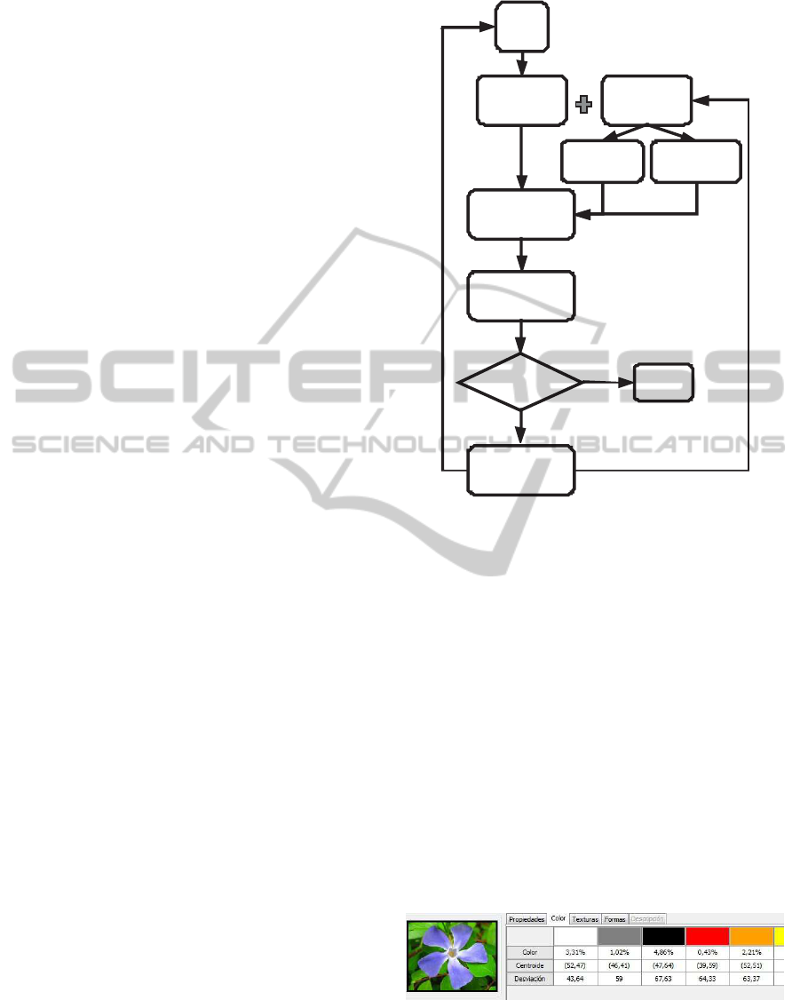
with a high percentage of success. The complete pro-
cess appears in the figure 1. The features extraction
has been partially implemented on Qatris IManager
(Arias-Nicol´as et al., 2007a) and the parameter esti-
mations for the Bayesian probit regression model has
been obtained from WinBUGS.
2.1 Feature Extraction
Numeric variables must be defined to represent the
image features. Then, the objective will be to set
a rule to classify the images in separated regions
by considering their features (Jai et al., 2000) and
(Sch¨urmann, 1996). Three different kind of features
are considered: color, texture and shape (Chor´as,
2003).
• Color. We looked for a color model similar to the
human perception. The one based on Hue, Satu-
ration and Luminosity (HSL) seems to be suitable
for this purpose (Smith, 1978). The 15 main col-
ors that we use are (de la Escalera, 2001): white,
grey, black, red, red-yellow, yellow, yellow-green,
green, green-cyan, cyan, cyan-blue, blue, blue-
pink, pink and pink red.
• Texture. Two methods are used to extract tex-
ture features. The first one is based on the gray
level co-ocurrence matrix (Haralick and Shapiro,
1993). The second method detects linear texture
Data
matrix
Difference
matrix
Prior
information
Classification
rule
Informative
Weakly
informative
Supervision
Newimages
areclassified
Stopping
criteria
End
Yes
No
Figure 1: Complete process.
primitives and uses the run length matrix (Gal-
loway, 1975).
• Shape. This features are based on the methods
proposed by (Belkasim et al., 1991). We use
Hu’s moments (first and second moments), cen-
troid (center of gravity), angle of minimum iner-
tia, area, perimeter, ratio of area and perimeter,
and major and minor axis of fitted ellipse.
In order to extract these features Qatris Iman-
ager software is used (Arias-Nicol´as et al., 2007a)
and (Arias-Nicol´as and Calle-Alonso, 2010). It has
been developed by SICUBO (spin-off of the Univer-
sity of Extremadura) with the cooperation of the re-
search groups DIB (Decisi´on e Inferencia Bayesiana)
and GIM (Grupo de Ingenier´ıa de Medios) from the
University of Extremadura. An example of the color
features used is shown in the figure 2.
Figure 2: Color features.
2.2 Pairwise Comparison Method
The pairwise comparison method begins after the ex-
ICPRAM 2012 - International Conference on Pattern Recognition Applications and Methods
468

traction of the features. We start with r images and
the values for each feature is saved in the data ma-
trix A, so we have r features vectors a
1
, . . . , a
r
. This
method compares every pair of images to obtain a ma-
trix of differences Λ. This matrix is used later in the
Bayesian regression.
Let d
k
be the difference function between images
for the k-feature, with k = 1, . . . , K. For each pair of
images (a
i
, a
j
) the values for the independent vari-
ables are computed as:
x
a
i
a
j
= (d
1
(a
i
, a
j
), d
2
(a
i
, a
j
), . . . , d
K
(a
i
, a
j
)). (1)
The response variable is defined as:
y
a
i
a
j
=

0, If images belongs to the same class,
1, If images belongs to different classes.
(2)
Now we can define the matrix of diferences Λ. It
contains (for every pair of images) the value of the in-
dependent variable, the differences between the fea-
tures and, if a regression model with constant is re-
quired, a row of 1’s.
Λ =








y
a
1
a
2
y
a
1
a
3
. . . y
a
r−1
a
r
1 1 . . . 1
d
1
(a
1
a
2
) d
1
(a
1
a
3
) . . . d
1
(a
r−1
a
r
)
d
2
(a
1
a
2
) d
2
(a
1
a
3
) . . . d
2
(a
r−1
a
r
)
.
.
.
.
.
. . . .
.
.
.
d
K
(a
1
a
2
) d
K
(a
1
a
3
) . . . d
K
(a
r−1
a
r
)








.
(3)
The Bayesian binary regression is applied with
these data. The objective is classify new images in
their respective classes. With this method any kind
of classification problem could be solved. It doesn’t
matter the number of classes.
2.3 Bayesian Regression
Let π and β be defined as:
π
a
i
a
j
= F(β
T
x
a
i
a
j
), (4)
β = (β
1
, β
2
, . . . , β
K
)
T
, (5)
with F(·) being a cumulative distribution function,
and β the regression parameters vector. A bi-
nary regression model is considered, so the indepen-
dent variable follows a Bernoulli distribution y
a
i
a
j
∼
Bernoulli(π
a
i
a
j
). In order to select the specific regres-
sion model, a model choice approach based on the
DIC (Deviance Information Criterion, (Spiegelhalter
et al., 2002)) has been performed. We have consid-
ered eight different regression models with symmet-
ric and asymmetric links. The probit model is usually
the one which obtains the lowest DIC and the best fit
for the data. Therefore, the probit model (McCullagh
and Nelder, 1989) is considered, i.e.:
π
a
i
a
j
= F(β
T
x
a
i
a
j
) = Φ(β
T
x
a
i
a
j
), (6)
being Φ the standard normal cumulative distribution
function.
In the Bayesian regression model, the coefficients
are random variables. Firstly, the method is applied
with no prior information, so a weakly informative
prior distribution for the parameters is used (Zellner
and Rossi, 1994). Specifically, a normal prior distri-
bution with mean equal to zero and high variances (to
let the parameters vary in a large range) is considered.
Since our objective is to determine a measurement
of discrepancy among images, and as the independent
variables are non-negative, the predictor will be non-
negative. Then, the parameters of the model should
be non-negative. In order to achieve this goal, a trun-
cated normal in the interval [0, u], with mean µ and
variance σ
2
can be considered. Then, the cumulative
distribution function is:
F(x) =





0 x < 0,
Φ(
√
σ(x−µ))−Φ(
√
σ(−µ))
Φ(
√
σ(u−µ))−Φ(
√
σ(−µ))
0 < x < u,
1 x > u.
(7)
In order to estimate the parameters, Markov Chain
Monte Carlo (MCMC) methods are implemented by
using the software WinBUGS (Chen et al., 2000). We
have to simulate a long chain to achieve convergence.
Then, we discart the first iterations and use the rest to
estimate the regression parameters.
After the coefficients have been estimated, any
new image a
new
could be classified. The method au-
tomatically obtains all the pairwise comparisons be-
tween a
new
and any other a
i
. With these values we
can estimate every y
a
new
a
i
for i in 1 to r by discretiz-
ing:
π
a
new
a
i
= Φ(β
T
x
a
new
a
i
). (8)
Finally, we use a decision criterion to assign a
class to every image. The nearest neighbors method
(Fix and Hodges, 1951) is used, so we find the N low-
est values of y and their corresponding images. We
can assign the new image to the class with highest
frequency among the images selected.
2.4 Relevance Feedback
Now, we can classify new images using the method
based on a weakly informative prior distribution, but
the objective is to use the information achieved in the
experiments to improve the results. The supervision
of an expert is needed in the last stage of the method.
BAYESIAN SUPERVISED IMAGE CLASSIFICATION BASED ON A PAIRWISE COMPARISON METHOD
469

When some new images are classified automati-
cally, they can be in the correct class or not because
the system is not free of errors. To improve the classi-
fication and provide high quality results an expert may
help supervising the new images that have just been
evaluated. The information of the belonging class can
be added to the data used in the method. First we
make all the possible pairs between the initial images
and the new ones and we add y = 0 if the two images
compared are in the same class or y = 1 if they belong
to a different class. The new pairs and their differ-
ences are incorporated to the data matrix and will be
important in the next estimation of the model param-
eters.
However, there is more information we can pro-
vide from this results. The first time the parameter
estimation (made with the training sample of images)
is performed, a weakly informative prior distribution
is used. Later, the posterior distribution is studied.
The information obtained about this distribution is set
as the new prior distribution for the next stage and the
results should “learn” from the past experiment.
This interactive learning process let us to update
the parameters β of the model in a continuous way
and both the new data supervised by the expert and
the new information from the distribution will con-
tinue improving the results until the process has learnt
enough to be applied in an completely automatic way.
3 ILLUSTRATIVE EXAMPLES
3.1 Sports Images
In order to illustrate the method we show a simple
example of image classification. We have to classify
sport images from TV into two classes: football or
handball. To simplify and without loss of generality,
in this example we will use only 15 color percent-
age independent variables. The objective is to classify
correctly the images obtained from TV to know which
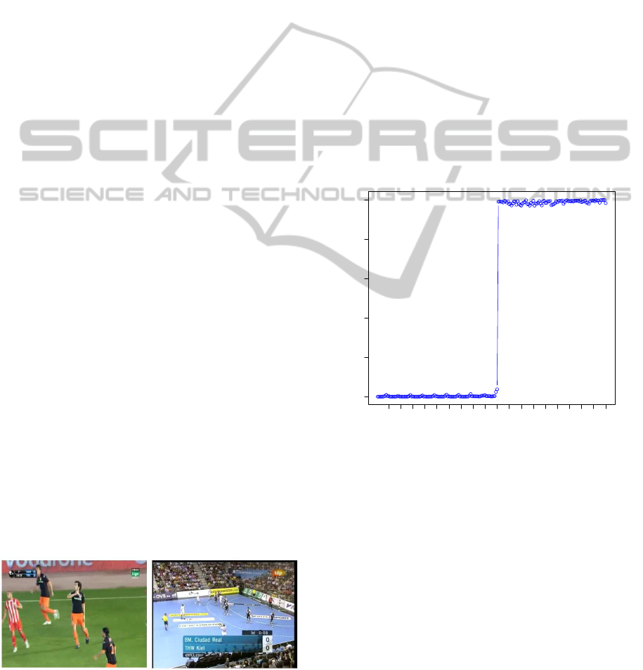
sport is appearing at every moment. Two images that
represent each class are shown in the figure 3.
Figure 3: Representative images of handball and football.
We start training the system with 20 images, 10 of
each class. Let a
1
, a
2
, . . . , a
10
be football images and
b
1
, b
2
, . . . , b
10
handball ones. By using Qatris Iman-
ager, we extract the color features. Then, every pair
of images is evaluated to obtain the distance between
them (190 pairs). Also, the classification value is as-
signed to each class, either y = 0 when both images
are from the same class, or y = 1 if one image is foot-
ball and the other is handball. Finally a weakly infor-
mative prior distribution is considered for the regres-
sion parameters.
The simulation is performed by using WinBUGS.
In order to achieve convergence 100,000 iterations
are simulated, burning the first 90,000. With the last
10,000 iterations, we estimate the parameters β for
the Bayesian probit model. With these estimations,
we can compute the value of ˆy. These values can be
compared with the real ones, because the classifica-
tion of these images is well known. As it can be seen
in Figure 4, all the estimations for training data are
correct, because the real values are one hundred times
y = 0 and ninety y = 1.
10 30 50 70 90 110 130 150 170 190
0.0 0.2 0.4 0.6 0.8 1.0
Comparaciones
Estimaciones
Figure 4: Values ˆy computed.
With the estimation of parameters of the model
we can classify any new image. In this case we will
choose 10 new images to be classified and, to test the
method, we already know their classification. We will
study five new football images a
11
, a
12
, . . . , a
15
and
five handball images b
11
, b
12
, . . . , b
15
.
First we form all possible pairs between the new
images and the old ones to obtain the differences ma-
trix. With this matrix and the estimation of β we
can compute the values of ˆy. These values are ar-
ranged from lowest to highest and, following the near-
est neighbor criterion, we study the ten images more
similar to each new image. Two images are more sim-
ilar as their corresponding value of y gets closer to
zero. For example, we can see in the table 1 the ten
ICPRAM 2012 - International Conference on Pattern Recognition Applications and Methods
470

Table 1: Ten most similar images to a
11
and b
11
.
a
11
a
5
a
2
a
7
a
4
a
6
a
1
a
3
a
8
a
10
a
9
b
11
b
10
b
9
b
2
b
1
b
3
b
5
b
4
b
8
b
6
b
7
most similar images to the new a
11
and b
11
.
The ten images closest to a
11
are football images,
and to b
11
are handball images, so we can classify
them in those classes. By following the same process
for all the new images, we obtain a perfect classifica-
tion. All the new images are classified into their cor-
rect class and there is no need to continue improving
the method with the supervision.
In other problems, there could be some mistakes.
At that moment, the expert should start the supervi-
sion. When the new images are supervised and cor-
rected (if there is any error), they are moved into the
data matrix to be used in the next stages of the pro-
cedure, constructing the classification rule. This way
to proceed is really valuable, since by providing the
opinion of an expert, the model can be guided in the
correct direction.
But there is still some information we can take ad-
vantage of. The estimation of β gives us the oppor-
tunity to study its posterior distribution. As a result
we estimate the distribution function for each param-
eter and incorporate them to the model as a prior dis-
tribution. For example, for β
1
we estimate a normal
distribution with mean 2.0608 and variance 0.3389.
The system continues receiving images and in ev-
ery stage it classifies and learns from the expert and
from the posterior distribution of the previous stage.
Actually, the expert only needs to supervise the re-
sults a few times until the method learns how to clas-
sify correctly, then it will do a completely automatic
classification.
3.2 Breast Tissue Classification
Our method is not only useful for images with the fea-
tures described before, we can use it to classify any
kind of data. In order to prove it, a real experiment
is evaluated. In this problem (Estrela da Silva et al.,
2000), the authors try to classify 106 patients, with
the results of a spectroscopy test, into 6 classes. This
type of test to diagnose breast cancer has the great ad-
vantages to be a minimally invasive technique, very
easy to use and also inexpensive. Significant differ-
ences of breast tissue were found by (Jossinet, 1998)
using this technique, so breast cancer could be fairly
detected with the Electrical Impedance Spectroscopy
(EIS).
Breast tissue was sampled from 106 patients un-
dergoing breast surgery. The nine features used are
extracted from Argand plot. Four of them were pre-
viously defined and studied statistically (Jossinet and
Lavandier, 1998):
• I
0
: Impedivity at zero frequency.
• PA
500
: Phase angle at 500kHz.
• S
HF
: High frequency slope of phase angle (at 250,
500 and 1000 kHz).
• D
A
: Impedance distance between spectral ends.
The other five features were newly presented in
the article (Estrela da Silva et al., 2000):
• Area: Area under spectrum.
• Area
DA
: Area normalised by D
A
.
• IP
MAX
: Maximum of the spectrum.
• D
R
: Distance between I
0
and real part of the max-
imum frequency point.
• Perim: Length of spectral curve.
There are six tissue classes, including three nor-
mal and three pathological. We will try to discrimi-
nate all of them, but with special attention to carci-
noma.
1. Connective tissue (normal).
2. Adipose tissue (normal).
3. Glandular tissue (normal).
4. Carcinoma (pathological).
5. Fibro-adenoma (pathological).
6. Mastopathy (pathological).
The authors found that it was difficult to solve the
problem with six classes together. As a solution they
selected a specific method to try to achieve their goal.
It was a hierarchical approach (Swain and Hauska,
1977) using linear discriminant analysis. First, they
obtained a 66.37% of general efficiency when classi-
fying six classes (see the reference column in table
2).
Table 2: Classification of breast tissue in six classes.
1st Iteration 2nd Iteration Reference
Carcinoma 95.24 95.24 81.82
Fibro-adenoma 40.00 46.67 66.67
Mastopathy 83.33 83.33 16.67
Glandular 56.25 62.50 54.54
Connective 100 100 85.71
Adipose 100 100 90.91
Average 79.14 81.29 66.37
As the results were poor for six classes, they tried
to classify different groups of classes, concluding that
the most important was to discriminate carcinoma
from fibro-adenoma + mastopathy + glandular tissue.
BAYESIAN SUPERVISED IMAGE CLASSIFICATION BASED ON A PAIRWISE COMPARISON METHOD
471

In this particular problem, they obtained a percent-
age higher than the previous one: 92.21% overall ef-
ficiency and 86.36% for carcinoma discrimination, as
it is shown in the reference column of table 3.
With our method we try to solve both the six
classes and the two classes problems. We use just the
same data from the article mentioned to compare the
results obtained. First we take the data matrix and
we compute the differences between all the cases (as
mentioned in section 2.2). The result is a new matrix
with 5565 rows and 9 features variables. One extra
variable is added to indicate if the cases compared in
each row belongs to the same class or not.
In the first stage a weakly informative Gaussian
distribution is used, because we don’t have any initial
information. With the estimations of the parameters
for the probit model, we obtain a value from 0 to 1
indicating their similarity for every pair of case. We
want to see if every case is well classified, so for each
one we select the top ten similar cases and the most
repeated class within this ten is the class assigned to
the case studied (nearest neighbor algorithm).
As we propose an interactive learning algorithm,
in this experiment we use the posterior distribution
of the parameters from an stage to include it as the
prior distribution for the next one. The method will
be learning and adapting every time the process is re-
peated. The number of iterations is not fixed at the
beginning, so we could compute it until the objective
efficiency is achieved.
We start by classifying all the cases into six
classes. One solution could be to classify first only
between normal or pathological, and then try to iden-
tify the specific class. We do it with all the classes
at the same time and then we can teach the system to
learn from its errors. As Estrela da Silva et al. present
in their paper, the most difficult classes to discrimi-
nate are fibro-adenoma and mastopathy. The results
in table 2 show this fact. In the first iteration we ob-
tain only a 40% correct classification. This is the low-
est classification efficiency in the six classes. On the
other hand we obtain a perfect classification of con-
nective and adipose tissues and very high percentages
for carcinoma (95.24%) and mastopathy (83.33%).
The overall efficiency is higher than the one of ref-
erence: 79.14% facing 66.37%.
After this first iteration, we have executed the
problem once, so the method will be improved with
the information we have now. In the next iteration,
the information about the parameters of the model
is included as prior information and the results of
right classified cases increase. We appreciate that the
classes that already had a good classification skill re-
main the same but the two lowest values of classifica-
tion improve their results. Fibro adenoma goes from
40% to 46.67%, and glandular tissue from 56.25%
to 62.50%. With this percentage rising we obtain an
overall efficiency of 81.29%, much higher than the
66.37% presented by the other authors. Also the most
important class, carcinoma, achieve a 95.24% of cor-
rect classified cases against the 81.82% reached in the
reference paper.
If we set a stopping criterion, the process will stop
when it is reached. For example, if we want at least
an overall 80% of efficiency and over 90% for carci-
noma class we have achieved this with two iterations.
This feedback has only been performed with the train-
ing data in order to compare the results with the ones
from other authors (see (Jossinet, 1998), (Jossinet and
Lavandier, 1998) and (Estrela da Silva et al., 2000)).
If new cases appear, the system would have more in-
formation and the relevance feedback could be even
greater than the one performed.
In order to conclude, we show the results in ta-
ble 3 for a situation with two classes: carcinoma and
fibro-adenoma + mastopathy + glandular. In the first
iteration we achieve the 100% correct classifications,
so we stop here and there is no need to improve the
method with some new iterations. In comparison with
the results obtained by Estrela da Silva et al., all the
percentages are improved.
Table 3: Classification of breast tissue in two classes.
Carcinoma Others Percent correct Reference
Carcinoma 21 0 100 86.36
Others 0 49 100 94.54
Total 21 49 100 92.21
4 CONCLUSIONS
In this paper we have proposed a novel pairwise com-
parison method based on a Bayesian regression to
classify automatically. By extracting color, texture
and shape features from the digital images, fair re-
sults are obtained for some real pattern recognition
problems. The method classifies any new cases and
improve the results every time it is executed again,
thanks to the relevance feedback. This interactive
methodology increases the quality of the results with
the supervision of an expert and the readjustment of
the prior distribution for the parameters of the model.
ACKNOWLEDGEMENTS
This research was partially supported by projects
ICPRAM 2012 - International Conference on Pattern Recognition Applications and Methods
472

TIN2008-06796-C04-03 and MTM2011-28983-C03-
02 from Ministerio de Ciencia e Innovaci´on, and
project GRU10100 from Junta de Extremadura.
REFERENCES
Arias-Nicol´as, J. P. and Calle-Alonso, F. (2010). A
novel content-based image retrieval system based
on bayesian logistic regression. In 18th Inter-
national Conference in Central Europe on Com-
puter Graphics, Visualization and Computer Vi-
sion’2010 (WSCG’2010) Poster proceedings, pages
19–22, PLZEN, Czech Republic. UNION Agency,
Science Press.
Arias-Nicol´as, J. P., Calle-Alonso, F., and Horrillo-Sierra,
I. (2007a). Qatris imanager, un sistema cbir basado
en regresi´on log´ıstica. Bolet´ın de Estad´ıstica e Inves-
tigaci´on Operativa, 23(2):9–13.
Arias-Nicol´as, J. P., P´erez, C. J., and Mart´ın, J. (2007b). A
logistic regression-based pairwise comparison method
to aggregate preferences. Group Decision and Nego-
tiation, 17(3):237–247.
Belkasim, S. O., Shridhar, M., and Ahmadi, M. (1991).
Pattern recognition with moment invariants: A com-
parative study and new results. Pattern Recognition,
24(12):1117–1138.
Chen, M. H., Spiegelhalter, D., Thomas, A., and Best,
N. (2000). The BUGS Project. MRC Bio-
statistics Unit, Cambridge, UK, http://www.mrc-
bsu.cam.ac.uk/bugs/winbugs/contents.shtml.
Chor´as, R. S. (2003). Content-based retrieval using color,
texture and shape information. Lecture Notes in Com-
puter Sciences, 2905:619–626.
de la Escalera, A. (2001). Visi´on por Computador, Funda-
mentos y M´etodos. Prentice-Hall.
El-Naqa, I., Yang, Y., Galatsanos, N. P., Nishikawa, R. M.,
and Wernick, M. N. (2004). A similarity learning ap-
proach to content-based image retrieval: application
to digital mammography. IEEE Transactions on Med-
ical Imaging, 23(10):1233–1244.
Estrela da Silva, J., Marques de S´a, J. P., and Jossinet, J.
(2000). Classification of breast tissue by electrical
impedance spectroscopy. Medical and Biological En-
gineering and Computing, 38:26–30.
Fix, E. and Hodges, J. L. (1951). Discriminatory analy-
sis, nonparametric discrimination consistency proper-
ties. Technical Report 4, USAF School of Aviation
Medicine.
Galloway, M. M. (1975). Texture analysis using grey level
run lengths. Computer Graphics and Image Process-
ing, 4:172–179.
Haralick, R. M. and Shapiro, L. G. (1993). Computer and
Robot Vision Vol.I. Addison-Wesley.
Jai, A. K., Duin, R., and Mao, J. (2000). Statistical pattern
recognition: A review. IEEE Transaction on pattern
and machine intelligence, 22(1):4–37.
Jossinet, J. (1998). The impedivity of freshly excised hu-
man breast tisue. Physiology Measures, 19:61–75.
Jossinet, J. and Lavandier, B. (1998). The discrimina-
tion of excised cancerous breast tissue samples us-
ing impedance spectroscopy. Bioelectrochemistry and
bioenergetics, 45:161–167.
McCullagh, P. and Nelder, J. A. (1989). Generalized Lineal
Models. Monographs on Statistics and Applied Prob-
ability. Chapman and Hall.
Sch¨urmann, J. (1996). Pattern Classification: A Unified
View of Statistical and Neural Approaches. Wiley and
sons.
Smeulders, A., Worring, M., Santini, S., Gupta, A., and
Jain, R. (2000). Content-based image retrieval at the
end of the early years. IEEE Transactions on Pat-
tern Analysis and Machine Intelligence, 22(12):1349–
1380.
Smith, A. R. (1978). Color gamut transform pairs. SIG-
GRAPH’78 Proceedings of the 5th annual conference
on Computer graphics and interactive techniques,
pages 12–19.
Spiegelhalter, D. J., Best, N. G., Carlin, B. P., and van der
Linde, A. (2002). Bayesian measures of model com-
plexity and fit (with discussion). Journal of the Royal
Statistical Society, Series B (Statistical Methodology),
64(4):583–639.
Swain, P. H. and Hauska, H. (1977). The decision tree clas-
sifier: design andpotential. IEEE Transaction on Geo-
science and remote Sensing, GE-15:142–147.
Theodoridis, S. and Koutroumbas, K. (2003). Pattern
Recognition. Elsevier Academia, 4th edition.
Tversky, A. (1977). Features of similarity. Psychological
Review, 84(4):327–352.
Zellner, A. and Rossi, P. (1994). Bayesian analysis of
dichotomous quantal response models. Journal of
Econometrics, 25(3):365–393.
BAYESIAN SUPERVISED IMAGE CLASSIFICATION BASED ON A PAIRWISE COMPARISON METHOD
473