
HYPERSPECTRAL UNMIXING WITH SIMULTANEOUS
DIMENSIONALITY ESTIMATION
Jos´e M. P. Nascimento
1
and Jos´e M. Bioucas-Dias
2
1
Instituto de Telecomunicac¸˜oes and Instituto Superior de Engenharia de Lisboa
R. Conselheiro Em´ıdio Navarro, N. 1, 1959-007 Lisboa, Portugal
2
Instituto de Telecomunicac¸˜oes and Instituto Superior T´ecnico, Technical University of Lisbon
Av. Rovisco Pais, Torre Norte, Piso 10, 1049-001 Lisboa, Portugal
Keywords:
Blind hyperspectral unmixing, Minimum volume simplex, Minimum Description Length (MDL), Variable
splitting augmented Lagrangian, Dimensionality reduction.
Abstract:
This paper is an elaboration of the simplex identification via split augmented Lagrangian (SISAL) algorithm
(Bioucas-Dias, 2009) to blindly unmix hyperspectral data. SISAL is a linear hyperspectral unmixing method of
the minimum volume class. This method solve a non-convex problem by a sequence of augmented Lagrangian
optimizations, where the positivity constraints, forcing the spectral vectors to belong to the convex hull of the
endmember signatures, are replaced by soft constraints.
With respect to SISAL, we introduce a dimensionality estimation method based on the minimum description
length (MDL) principle. The effectiveness of the proposed algorithm is illustrated with simulated and real
data.
1 INTRODUCTION
Although, there have been significant improvements
in the hyperspectral remote sensing sensors, there
are in an image pixels than contain more than one
material, i.e., the acquired spectral vectors are mix-
tures of the material spectral signatures present in
the scene (Bioucas-Dias and Plaza, 2010; Nascimento
and Bioucas-Dias, 2005a).
The linear mixing assumption has been widely
used to describe the observed hyperspectral vectors.
According to this assumption, a mixed pixel is a lin-
ear combination of endmembers signatures weighted
by the corresponding abundance fractions. Due to
physical considerations, the abundance fractions are
subject to the so-called non-negativity and a full-
additivity constraints (Bioucas-Dias and Plaza, 2010).
Hyperspectral unmixing, aims at estimating the
number of reference materials, also called endmem-
bers, their spectral signatures, and their abundance
fractions (Keshava and Mustard, 2002).
Approaches to hyperspectral linear unmixing can
be classified as either statistical or geometrical. Sta-
tistical methods very often formulate the problem
under the Bayesian framework (Nascimento and
Bioucas-Dias, 2011; Dobigeon et al., 2009; Arngren
et al., 2009; Moussaoui et al., 2008).
The geometric perspective just referred to has
been exploited by many algorithms. These algorithms
are based on the fact that, under the linear mixing
model, hyperspectral vectors belong to a simplex set
whose vertices correspond to the endmembers signa-
tures. Therefore, finding the endmembers is equiva-
lent to identifying the vertices of the referred to sim-
plex (Nascimento and Bioucas-Dias, 2005b).
Some algorithms assume the presence of, at least,
one pure pixel per endmember (i. e., containing just
one material). Some popular algorithms taking this
assumption are vertex component analysis (VCA),
(Nascimento and Bioucas-Dias, 2005b), the auto-
mated morphological endmember extraction (AMEE)
(Plaza et al., 2002), the pixel purity index (PPI),
(Boardman, 1993), and the N-FINDR (Winter, 1999)
(see (Chan et al., 2011) for recently introduced rein-
terpretations and improvements of N-FINDR). These
methods are followed by a fully constrained least
square estimation (Heinz and Chein-I-Chang, 2001)
or by a maximum likelihood estimation (Settle, 1996)
of the abundance fractions to complete the unmixing
procedure.
If the pure pixel assumption is not fulfilled, which
is a more realistic scenario, the unmixing process
is a rather challenging task, since some endmem-
bers are not in the dataset. Some recent methods,
438
M. P. Nascimento J. and M. Bioucas-Dias J..
HYPERSPECTRAL UNMIXING WITH SIMULTANEOUS DIMENSIONALITY ESTIMATION.
DOI: 10.5220/0003877504380444
In Proceedings of the 1st International Conference on Pattern Recognition Applications and Methods (PRARSHIA-2012), pages 438-444
ISBN: 978-989-8425-98-0
Copyright
c
2012 SCITEPRESS (Science and Technology Publications, Lda.)
in the vein of Craig’s work minimum Volume Trans-
form (MVT) (Craig, 1994) which finds the smallest
simplex that contain the dataset, are the iterated con-
strained endmember (ICE), (Berman et al., 2004), the
minimum volume simplex (MVSA) (Li and Bioucas-
Dias, 2008), the Minimum-Volume Enclosing Simplex
Algorithm (MVES) (Chan et al., 2009), and the alter-
nating projected subgradients (APS) (Zymnis et al.,
2007).
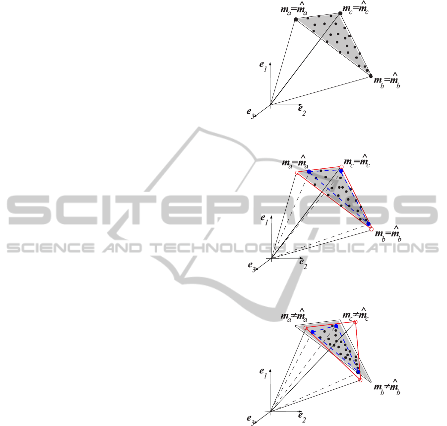
Fig. 1 illustrates three datasets raising different
degrees of difficulties in what unmixing is concerned:
the dataset shown in Fig.1(a) contains pure pixels, i.e.,
the spectra corresponding to the simplex vertices are
in the dataset. This is the easiest scenario with which
all the unmixing algorithms cope without problems;
the dataset shown in Fig.1(b) does not contain pure
pixels, at least for some endmembers. This is a much
more challenging, usually attacked with the minimum
volume based methods, note that pure-pixels based
methods are outperformedunder these circumstances;
Fig.1(c), contains a highly mixed dataset where only
statistical methods can give accurate unmixing re-
sults.
Most of these methods assume that the number of
endmembers are knowna-priori or estimated for some
method, such as, NWHFC (Chang and Du, 2004),
HySime (Bioucas-Dias and Nascimento, 2008), and
Second moment linear dimensionality (SML) (Ba-
jorski, 2011). The robust signal subspace estimation
(RSSE) (Diani and Corsini, 2010) have been proposed
in order to estimate the signal subspace in the pres-
ence of rare signal pixels, thus it can be used as a
preprocessing step for small target detection appli-
cations. Sparsity promoting ICE (SPICE) (Zare and
Gader, 2007) is an extension of ICE algorithm that
incorporates sparsity-promoting priors to find the cor-
rect number of endmembers. The framework pre-
sented in (Broadwater et al., 2004) also estimates the
number of endmembers when it unmix the data. This
framework has the disadvantage of using the Unsu-
pervised Fully Constrained Least Squares (UFCLS)
algorithm proposed in (Heinz and Chein-I-Chang,
2001) which assumes the presence of at least one pure
pixel per endmember.
Simplex identification via split augmented La-
grangian (SISAL) (Bioucas-Dias, 2009) belongs to
the minimum volume class methods. The non-convex
optimization problem is solved as a sequence of non-
smooth convex subproblems using variable splitting
to obtain a constraint formulation, and then applying
an augmented Lagrangian technique.
This paper proposes an improvement of SISAL
by introducing an algorithm based on the minimum
description length (MDL) principle. Thus, SISAL is
(a)
(b)
(c)
Figure 1: Illustration of tree scenarios: (a) with pure pixels
(solid line - estimated simplex by all methods); (b) with-
out pure pixels and with pixels in the facets (solid red line
- estimated simplex based on minimum volume; dashed
blue line - estimated simplex by pure-pixel based methods);
(c) highly mixed pixels (solid red line - estimated simplex
based on minimum volume; dashed blue line - estimated
simplex by pure-pixel based methods).
able to estimate the number of endmembers as it un-
mix the hyperspectral dataset.
This paper is organized as follows. Section 2
describes the fundamentals of the proposed method.
Section 3 presents the method to infer the number
of number of endmembers. Section 4 illustrates as-
HYPERSPECTRAL UNMIXING WITH SIMULTANEOUS DIMENSIONALITY ESTIMATION
439

pects of the performance of the proposed approach
with experimental data based on U.S.G.S. laboratory
spectra and with real hyperspectral data collected by
the AVIRIS sensor, respectively. Section 5 concludes
with some remarks.
2 PROBLEM FORMULATION
Assuming the linear observation model, each pixel
y of an hyperspectral image can be represented as a
spectral vector in R
l
(l is the number of bands) and is
given by y = Ms + n, where M ≡ [m
1
,m
2
,...,m
p
] is
an l × p mixing matrix (m
j
denotes the jth endmem-
ber spectral signature), p is the number of endmem-
bers present in the covered area, s = [s
1
,s
2
,...,s
p
]
T
is
the abundance vector containing the fractions of each
endmember (notation (·)
T
stands for vector trans-
posed), and vector n holds the sensor noise and mod-
eling errors.
To fix notation, let Y ≡ [y
1
, ...,y
n
] ∈ R
l×n
denote
a matrix holding the observed spectral vectors, S ≡
[s
1
, ...,s
n
] ∈ R
p×n
a matrix holding the respective
abundance fractions, and N ≡ [n
1
, ...,n
n
] ∈ R
l×n
ac-
counts for additive noise. To be physically meaning-
ful, abundance fractions are subject to non-negativity
and constant sum constraints, i.e., {s ∈ R
p
: s
0,1
T
p
s = 1
T
n
}
1
. Therefore
Y = MS+ N
s.t. : S 0, 1
T
p
S = 1
T
n
. (1)
Usually the number of endmembers is much lower
than the number of bands (p ≪ L). Thus, the observed
spectral vectors can be projected onto the signal sub-
space. The identification of the signal subspace im-
proves the SNR, allows a correct dimension reduc-
tion, and thus yields gains in computational time and
complexity (Bioucas-Dias and Nascimento, 2008).
Let E
p
be a matrix, with orthonormal columns,
spanning the signal subspace. Thus
X ≡ E
T
p
Y+ E
T
p
N
= AS+ N
∗
, (2)
where X ≡ [x
1
, ...,x
n
] ∈ R
p×n
denote a matrix hold-
ing the projected spectral vectors, A = E
T
p
M is a p× p
square mixing matrix, and N
∗
accounts for the pro-
jected noise.
Linear unmixing amounts to infer matrices A and
S. This can be achieved by fitting a minimum volume
simplex to the dataset (Craig, 1994). Finding a min-
imum volume matrix A subject to constraints in (1),
1
s 0 means s
j
≥ 0, for j = 1,... , p and 1
T
p
≡ [1,. . .,1]
leads to the non-convex optimization problem
b
Q = argmin
Q
{−log|detQ|}
s.t. : QX 0, 1
T
p
QX = 1
T
n
, (3)
where Q ≡ A
−1
. The constraint 1
T
p
QX = 1
T
n
can be
simplified, by multiplying the equality on the right
hand side by X
T
(XX
T
)
−1
, resulting 1
T
p
QX = 1
T
n
⇔
1
T
p
Q = a
T
, where a
T
≡ 1
T
n
X
T
(XX
T
)
−1
.
SISAL aims to give a sub-optimal solution of (3)
solving the following problem by a sequence of aug-
mented Lagrangian optimizations:
b
Q
∗
= argmin
Q
{−log|detQ| + λkQXk
h
}
s.t. : 1
T
p
Q = a
T
, (4)
where kQXk
h
≡
∑
ij
h(QX), h(x) ≡ max(−x,0) is
the so-called hinge function and λ is the regulariza-
tion parameter. Notice that kQXk
h
penalizes nega-
tive components of QX, thus playing the rule of a
soft constraint, yielding solutions that are robust to
outliers, noise, and poor initialization.(see (Bioucas-
Dias, 2009) for details).
3 NUMBER OF ENDMEMBERS
ESTIMATION
The MDL principle proposed by Rissanen (Rissanen,
1978) aims to select the model that offers the shortest
description length of the data. This approach can be
used to estimate the number of endmembers (Broad-
water et al., 2004). The well-known MDL criterion
for n i.i.d. observations, in general, is given by
b
k
MDL
= argmin
k
L (X|
b
θ
k
) +
1
2
klogn
, (5)
where L (X|
b
θ
k
) is a likelihood equation based on the
projected data X with parameters θ, and
1
2
klogn is
the penalizing term that increases with k (Figueiredo
and Jain, 2002).
Assuming that the additive noise is Gaussian dis-
tributed, i.e. n ∼ N (0,Λ)and given a set of n i.i.d.
observed samples, the likelihood equation is given by:
L (X|
b
θ
k
) ≡
n
∑
i=1
h
−log p(x
i
|
b
θ
k
)
i
=
n
2
plog(2π) + log| detΛ|
+
1
2
tr
h
(X− AS)
T
Λ
−1
(X− AS)
i
,
(6)
ICPRAM 2012 - International Conference on Pattern Recognition Applications and Methods
440
where tr(·) denotes the trace of a matrix, matrices A
and S are replaced by their estimates using SISAL al-
gorithm, the noise covariance matrix, Λ is estimated
using the algorithm based on the multiple regression
theory proposed in (Bioucas-Dias and Nascimento,
2008) and the number of free parameters is k = p
2
.
The resulting optimization algorithm is an iterative
scheme that requires to compute the objective func-
tion and to estimate the matrices A, S, and Λ for each
value of p.
4 EXPERIMENTS
This section provides simulated and real data experi-
ments to illustrate the algorithm’s performance. The
proposed method is tested and compared with SPICE
(Zare and Gader, 2007) on different simulated sce-
narios concerning with different signal-to-noise ratio
(SNR), absence of pure pixels, and number of end-
members present in the scene. The proposed method
is also applied to real hyperspectral data collected by
the AVIRIS sensor over Cuprite, Nevada.
4.1 Evaluation with Simulated Data
In this section the proposed method is tested on sim-
ulated scenes. To evaluate the performance of the al-
gorithm the spectral angle distance (SAD) (Keshava
and Mustard, 2002) is used. This widely known met-
ric measures the shape similarity between the ith end-
member signature m
i
and its estimate
b
m
i
. Based on
this metric we define a spectral root mean square an-
gle error, given by:
ε
m
≡
1
p
"
p
∑
i=1
arccos
m
T
i
b
m
i
km
i
kk
b
m
i
k
2
#
1/2
. (7)
To measure the similarity between the observed data
and the unmix result it is also computed the residual
error between the observed pixels and their estimates:
r
ls
≡ kY−
b
M
b
Sk
2
F
, (8)
where
b
M = E
p
b
A and
b
S are estimated by SISAL.
Concerning the simulated data creation a hyper-
spectral image composed of 10
4
pixels is generated
according to expression (1), where spectral signatures
where selected from the USGS digital spectral library.
The selection of endmember signatures is arbitrary
as long as they are linearly independent. The re-
flectances contain 224 spectral bands covering wave-
lengths from 0.38 to 2.5µm with a spectral resolution
0 0.5 1
0
0.2
0.4
0.6
0.8
1
channel 50 (λ = 827nm)
channel 150 (λ = 1780nm)
data
True endmembers
Estimated Endmembers
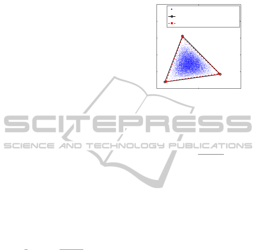
Figure 2: Scatterplot of the three endmembers mixture:
Dataset (blue dots); true endmembers (black circles); Pro-
posed method estimates (red squares).
of 10nm. The abundance fractions are generated ac-
cording to a Dirichlet distribution given by
D(s
1
, ..., s
p
|µ
1
, ..., µ
p
) =
Γ(
∑
p
j=1
µ
j
)
∏
p
j=1
Γ(µ
j
)
p
∏
j=1
s
µ
j
−1
j
,
(9)
where {s
1
,..., s
p
} are subject to non-negativity
and constant sum constraints. This density, be-
sides enforcing positivity and full additivity con-
straints, displays a wide range of shapes, depend-
ing on the parameters of the distribution µ =
[µ
1
,...,µ
p
]. In this experiment the Dirichlet param-
eters are set to µ = [3,. . . ,3], concerning the addi-
tive noise, the SNR, which is defined as SNR ≡
10log
10
E
y
T
y
/E
n
T
n
, is set to 30dB.
Fig. 2 presents a scatterplot of the simulated scene
for the p = 3 case, where dots represent the pixels
and circles represent the true endmembers. This Fig-
ure also shows the endmembers estimates (squares).
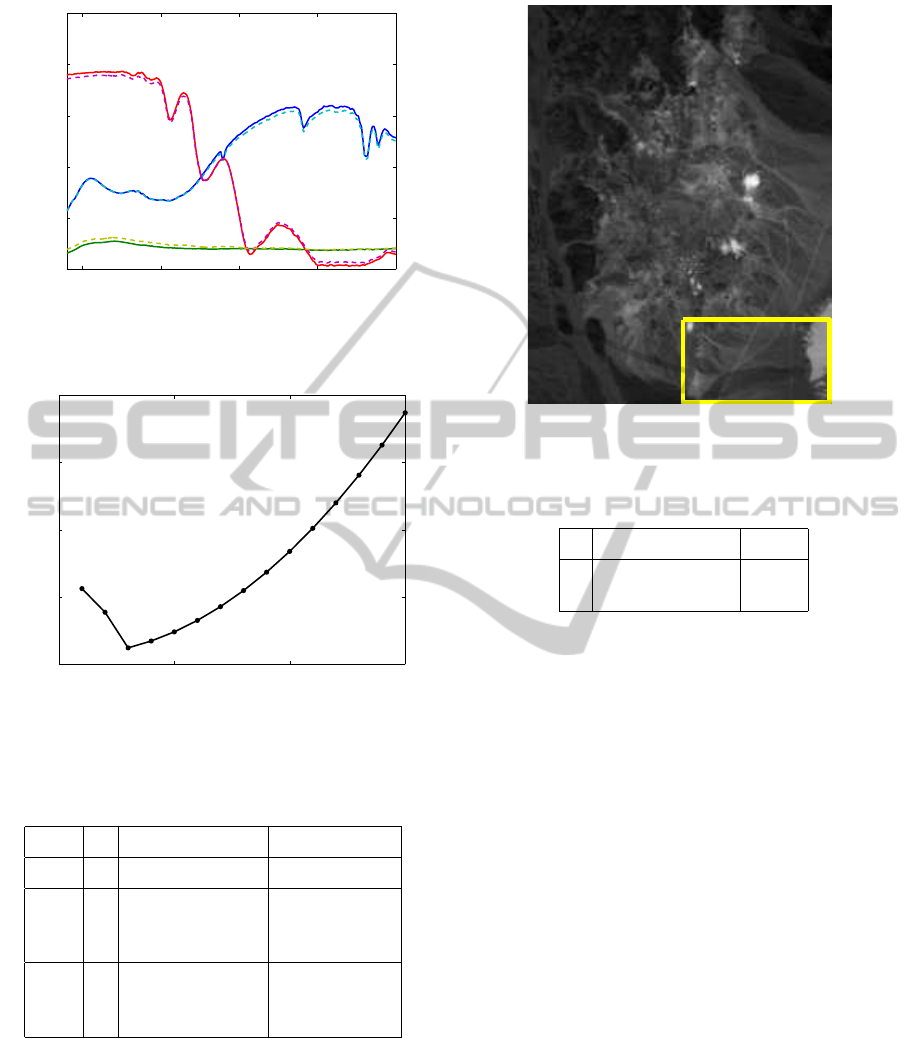
Fig.3 shows the endmembers signatures (solid line)
and their estimates (dashed line). Note that, in this
experiment there is no pure pixels in the dataset, how-
ever, the endmembers estimates are very close to the
true ones.
Fig 4, presents the evolution of the cost function
[see expression (5)] as a function of the number of
endmembers. The minimum of the function occurs at
b
k = 3 which is the true number of endmembers in the
scene.
Table 1 presents the root mean square error dis-
tance ε
m
, the residual least squares error r
ls
, and the
estimated number of endmembers for different exper-
iments where p is set to {3, 5,10} and the SNR is
set to {30,50} dB. Note that the estimated values are
exactly the number of endmembers in the scene and
HYPERSPECTRAL UNMIXING WITH SIMULTANEOUS DIMENSIONALITY ESTIMATION
441
0.5 1 1.5 2 2.5
0
0.2
0.4
0.6
0.8
1
Wavelength (nm)
Reflectances
Figure 3: Endmembers signatures (solid line) and their es-
timates (dashed line).
0 5 10 15
0
200
400
600
800
number of endmembers (p)
Cost function
Figure 4: Cost function evolution as a function of the num-
ber of endmembers.
Table 1: Results for different scenarios as a function of the
SNR and of the number of endmembers (p).
Proposed Method SPICE
SNR p
b
k ε
m
r
ls
b
k ε
m
r
ls
3 3 0.048 4.76 3 0.293 4.82
30dB 5 5 0.053 6.41 5 0.198 6.47
10 10 0.929 6.99 6 0.258 7.18
3 3 0.042 0.47 3 0.141 1.06
50dB 5 5 0.059 0.64 5 0.432 1.30
10 10 0.196 0.70 6 0.268 1.70
the unmix error increases with increasing values of p
and with noise level. The results achieved by SPICE
in terms of residual error are similar to the proposed
method results, although the errors between endmem-
bers signatures and their estimates are worst.
Figure 5: Band 30 (wavelength λ = 655.8nm) of the subim-
age of AVIRIS Cuprite Nevada dataset (rectangle denotes
the image fraction used in the experiment).
Table 2: Results for Cuprite dataset.
Proposed method SPICE
b
k 6 7
r
ls
3.13 3.27
4.2 Experiments with Real
Hyperspectral Data
In this section, the proposed method is applied to a
subset (50× 90 pixels and 224 bands) of the Cuprite
dataset acquired by the AVIRIS sensor on June 19,
1997, Fig. 5 shows band 30 (wavelength λ =
667.3nm) of the subimage of AVIRIS cuprite Nevada
dataset. The AVIRIS instrument covers the spectral
region from 0.41µm to 2.45µm in 224 bands with a
10nm band width. Flying at an altitude of 20km, it
has an IFOV of 20m and views a swath over 10km
wide. This site has been extensively used for remote
sensing experiments over the past years and its geol-
ogy was previously mapped in detail (Swayze et al.,
1992).
Table 2 present the residual error and the esti-
mated number of endmembers for SPICE and for the
proposed method. The results of both methods are
comparable.
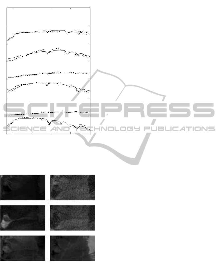
Fig.6 shows the estimated signatures, which are
compared with the nearest laboratory spectra, to vi-
sually distinguish the different endmembers an off-
set has been added to each signature. Note that, this
endmembers are known to dominate the considered
subimage (Swayze et al., 1992).
ICPRAM 2012 - International Conference on Pattern Recognition Applications and Methods
442
0.5 1 1.5 2 2.5
λ (µm)
a)
b)
c)
d)
e)
f)
Figure 6: Comparison of the estimated signatures (dashed
line) with the nearest USGS spectra (solid line): a) Alunite;
b) Desert vanish; c) Dumortierite; d) Sphene; e) Kaolinite;
f) Montmorillonite.
a)
b)
c)
d)
e)
f)
Figure 7: Abundance maps estimates: a) Alunite; b) Desert
vanish; c) Dumortierite; d) Sphene; e) Kaolinite; f) Mont-
morillonite.
Fig.7 presents the estimated abundance maps for
the extracted endmembers. A visual comparisonshow
that these maps are in accordance with the known
ground truth. Note that for this region Desert vanish
(Fig.7b)) and Sphene (Fig. 7d)) abundance maps are
very similar. These results show the potential of the
proposed method to simultaneously select the number
of endmembers, estimate the spectral signatures, and
their abundance fractions.
5 CONCLUSIONS
In this paper, a new method is proposed to blindly
unmix hyperspectral data and simultaneously infer
the number of endmembers based on the minimum
description length (MDL) principle. The endmem-
bers spectra estimates is based on SISAL algorithm
(Bioucas-Dias, 2009) which solves a non-convex
problem by a sequence of augmented Lagrangian op-
timizations. The experimental results achieved shows
the potential of the proposed method.
ACKNOWLEDGEMENTS
This work was supported by the Instituto de
Telecomunicac¸˜oes and by the Fundac¸˜ao para a
Ciˆencia e Tecnologia under project HoHus.
REFERENCES
Arngren, M., Schmidt, M. N., and larsen, J. (2009).
Bayesian Nonnegative Matrix Factorization with Vol-
ume Prior for Unmixing of Hyperspectral Images. In
Machine Learning for Signal Processing, IEEE Work-
shop on (MLSP).
Bajorski, P. (2011). Second Moment Linear Dimensional-
ity as an Alternative to Virtual Dimensionality. IEEE
Trans. Geosci. Remote Sensing, 49(2):672–678.
Berman, M., Kiiveri, H., Lagerstrom, R., Ernst, A., Dunne,
R., and Huntington, J. F. (2004). ICE: A Statistical
Approach to Identifying Endmembers in Hyperspec-
tral Images. IEEE Trans. Geosci. Remote Sensing,
42(10):2085– 2095.
Bioucas-Dias, J. M. (2009). A Variable Splitting Aug-
mented Lagrangian Approach to Linear Spectral Un-
mixing. In First IEEE GRSS Workshop on Hyperspec-
tral Image and Signal Processing-WHISPERS’2009.
Bioucas-Dias, J. M. and Nascimento, J. M. P. (2008).
Hyperspectral Subspace Identification. IEEE Trans.
Geosci. Remote Sensing, 46(8):2435–2445.
Bioucas-Dias, J. M. and Plaza, A. (2010). Hyperspec-
tral unmixing: geometrical, statistical, and sparse
regression-based approaches. volume 7830. SPIE.
Boardman, J. (1993). Automating Spectral Unmixing of
AVIRIS Data using Convex Geometry Concepts. In
Summaries of the Fourth Annual JPL Airborne Geo-
science Workshop, JPL Pub. 93-26, AVIRIS Work-
shop., volume 1, pages 11–14.
HYPERSPECTRAL UNMIXING WITH SIMULTANEOUS DIMENSIONALITY ESTIMATION
443

Broadwater, J., Meth, R., and Chellappa, R. (2004). Dimen-
sionality Estimation in Hyper-spectral Imagery Using
Minimum Description Length. In Proceedings of the
Army Science Conference, Orlando, FL.
Chan, T.-H., Chi, C.-Y., Huang, Y.-M., and Ma, W.-K.
(2009). A Convex Analysis-Based Minimum-Volume
Enclosing Simplex Algorithm for Hyperspectral Un-
mixing. IEEE Trans. Signal Processing, 57(11):4418
– 4432.
Chan, T.-H., Ma, W.-K., Ambikapathi, A., and Chi, C.-Y.
(2011). A simplex volume maximization framework
for hyperspectral endmember extraction. IEEE Trans.
Geosci. Remote Sensing, -(-):1 –17. in press.
Chang, C.-I. and Du, Q. (2004). Estimation of Number
of Spectrally Distinct Signal Sources in Hyperspec-
tral Imagery. IEEE Trans. Geosci. Remote Sensing,
42(3):608–619.
Craig, M. D. (1994). Minimum-volume Transforms for Re-
motely Sensed Data. IEEE Trans. Geosci. Remote
Sensing, 32:99–109.
Diani, N. A. M. and Corsini, G. (2010). Hyperspectral Sig-
nal Subspace Identification in the Presence of Rare
Signal Components. IEEE Trans. Geosci. Remote
Sensing, 48(4):1940–1954.
Dobigeon, N., Moussaoui, S., Coulon, M., Tourneret, J.-
Y., and Hero, A. O. (2009). Joint Bayesian Endmem-
ber Extraction and Linear Unmixing for Hyperspectral
Imagery. IEEE Trans. Signal Processing, 57(11):4355
– 4368.
Figueiredo, M. A. T. and Jain, A. K. (2002). Unsupervised
Learning of Finite Mixture Models. IEEE Trans. Pat-
tern Anal. Machine Intell., 44(3):381–396.
Heinz, D. and Chein-I-Chang (2001). Fully Constrained
Least Squares Linear Spectral Mixture Analysis
Method for Material Quantification in Hyperspectral
Imagery. Geoscience and Remote Sensing, IEEE
Transactions on, 39(3):529–545.
Keshava, N. and Mustard, J. (2002). Spectral Unmixing.
IEEE Signal Processing Mag., 19(1):44–57.
Li, J. and Bioucas-Dias, J. M. (2008). Minimum Volume
Simplex Analysis: A Fast Algorithm to Unmix Hy-
perspectral Data. In Proc. of the IEEE Int. Geosci. and
Remote Sensing Symp., volume 3, pages 250 – 253.
Moussaoui, S., Hauksd´ottir, H., Schmidt, F., Jutten, C.,
Chanussot, J., Brie, D., Dout´e, S., and Benediktsson,
J. A. (2008). On the Decomposition of Mars Hyper-
spectral Data by ICA and Bayesian Positive Source
Separation. Neurocomputing, 71(10-12):2194–2208.
Nascimento, J. M. P. and Bioucas-Dias, J. M. (2005a). Does
Independent Component Analysis Play a Role in Un-
mixing Hyperspectral Data? IEEE Trans. Geosci. Re-
mote Sensing, 43(1):175–187.
Nascimento, J. M. P. and Bioucas-Dias, J. M. (2005b). Ver-
tex Component Analysis: A Fast Algorithm to Un-
mix Hyperspectral Data. IEEE Trans. Geosci. Remote
Sensing, 43(4):898–910.
Nascimento, J. M. P. and Bioucas-Dias, J. M. (2011). Hy-
perspectral unmixing based on mixtures of dirichlet
components. IEEE Transactions on Geoscience and
Remote Sensing, pages –. in press.
Plaza, A., Martinez, P., Perez, R., and Plaza, J. (2002).
Spatial/Spectral Endmember Extraction by Multidi-
mensional Morphological Operations. IEEE Trans.
Geosci. Remote Sensing, 40(9):2025–2041.
Rissanen, J. (1978). Modeling by Shortest Data Descrip-
tion. Automatica, 14:465–471.
Settle, J. J. (1996). On the Relationship Between Spec-
tral Unmixing and Subspace Projection. IEEE Trans.
Geosci. Remote Sensing, 34:1045–1046.
Swayze, G., Clark, R., Sutley, S., and Gallagher, A.
(1992). Ground-Truthing AVIRIS Mineral Mapping
at Cuprite, Nevada. In Summaries of the Third Annual
JPL Airborne Geosciences Workshop, pages 47–49.
Winter, M. E. (1999). N-FINDR: An Algorithm for Fast
Autonomous Spectral End-member Determination in
Hyperspectral Data. In Proc. of the SPIE conference
on Imaging Spectrometry V, volume 3753, pages 266–
275.
Zare, A. and Gader, P. (2007). Sparsity Promoting Iterated
Constrained Endmember Detection in Hyperspectral
Imagery. IEEE Geosci. Remote Sensing Let., 4(3):446
– 450.
Zymnis, A., Kim, S.-J., Skaf, J., Parente, M., and Boyd, S.
(2007). Hyperspectral Image Unmixing via Alternat-
ing Projected Subgradients. In 41st Asilomar Confer-
ece on Signals, Systems, and Computer, pages 4–7.
ICPRAM 2012 - International Conference on Pattern Recognition Applications and Methods
444
