
PREDICTION FOR CONTROL DELAY
ON REINFORCEMENT LEARNING
Junya Saito, Kazuyuki Narisawa and Ayumi Shinohara
Graduate School of Information Sciences, Tohoku University, Sendai-shi, Japan
Keywords:
Machine learning, Reinforcement learning, Control delay, Markov decision process.
Abstract:
This paper addresses reinforcement learning problems with constant control delay, both for known case and
unknown case. First, we propose an algorithm for known delay, which is a simple extension of the model-free
learning algorithm introduced by (Schuitema et al., 2010). We extend it to predict current states explicitly, and
empirically show that it is more efficient than existing algorithms. Next, we consider the case that the delay is
unknown but its maximum value is bounded. We propose an algorithm using accuracy of prediction of states
for this case. We show that the algorithm performs as efficient as the one which knows the real delay.
1 INTRODUCTION
Reinforcement learning is one of the most active
research area of machine learning, where an agent
learns how to take appropriate actions in an environ-
ment so that it obtains the maximum cumulative re-
ward through observation and interaction. In many
cases, the Markov Decision Process (shortly MDP) is
used as a framework for reinforcement learning.
In real world applications, it is often the case that
time delay, called control delay between observation
and control matters seriously. For example, commu-
nication latency between controlling program and tar-
get robots may not be negligible, especially for slow
networks, such as Mars exploration project. Even for
a single agent, decision making including heavy com-
putations, e.g. image recognition, may cause action
delays.
Some researchers have investigated such situa-
tions, that is reinforcement learning with delay. Kat-
sikopilos et al. showed that the MDP with de-
lay can be reduced to the MDP without delay (Kat-
sikopoulos and Engelbrecht, 2003). Moreover, they
showed that delay for actions and delay for observa-
tions are equivalent from a view point of learner, al-
though these have been developed separately. Walsh
et al. proposed Model Based Simulation method,
in which they combined model-based reinforcement
learning and prediction of current states. Their algo-
rithm performs well even under the delay, although
it requires heavy computational resources (Walsh
et al., 2007). Schuitema et al. approached this prob-
lem by using model-free learning (Schuitema et al.,
2010). Their algorithm, called dSARSA(λ), is based
on Sarsa(λ) (Sutton and Barto, 1998), and it updates
Q-function with considering the delay. However, it
did not explicitly use the delay for selecting next ac-
tions. In this paper, weshow that the performancewill
increase if we add prediction of states in dSARSA(λ)
by some experiments.
Moreover, we also consider the case that the de-
lay is not known to the learner. We propose a simple
algorithm using accuracy of prediction of states, and
we verify that it works as efficient as the learner who
knows the real delay.
2 PRELIMINARIES
A Markov Decision Process (MDP) is a 4-tuple
hS, A, P, Ri, where S is a set of states, and A is a set of
actions. P: S× A× S → [0, 1] is a mapping indicating
the probability that the next state becomes s
′
∈ S when
an agent executes action a ∈ A in state s ∈ S. The re-
ward function R: S × A → ℜ defines the expected re-
ward that the agent obtains when taking action a ∈ A
in state s ∈ S. We assume that both S and A are finite
and discrete.
In this paper, we deal with control de-
lay (Schuitema et al., 2010), which is delay between
observation and control action. We refer to control
delay as delay below. Walsh et al. (Walsh et al., 2007)
proposed the constant delayed MDP (CDMDP),
579
Saito J., Narisawa K. and Shinohara A..
PREDICTION FOR CONTROL DELAY ON REINFORCEMENT LEARNING.
DOI: 10.5220/0003883405790586
In Proceedings of the 4th International Conference on Agents and Artificial Intelligence (SSML-2012), pages 579-586
ISBN: 978-989-8425-95-9
Copyright
c
2012 SCITEPRESS (Science and Technology Publications, Lda.)

which is an MDP with known constant delay. We
describe CDMDP as a 5-tuple hS, A, P, R, ki, where
k is a non-negative integer representing delay. We
are also interested in the situation that the delay is
unknown to the agents, although its maximum value
is known. We define an unknown constant delayed
MDP (UCDMDP) as a 5-tuple hS, A, P, R, k
max
i,
where k
max
is a non-negative integer that bounds
delay. The real value k of delay is not given to the
agent, but is fixed and satisfies 0 ≤ k ≤ k
max
.
3 dSARSA(λ)
k
: ALGORITHM
FOR KNOWN DELAY
Q-learning and Sarsa are popular on-line algorithms
which directly estimate the Q-function Q(s, a), that
calculates the quality of a state-action combination.
In order to accelerate convergence, eligibility traces
are often combined to Q-learning and Sarsa, (see,
e.g., (Sutton and Barto, 1998)) that is called Q(λ) and
Sarsa(λ), respectively.
Several approaches using Q(λ) and Sarsa(λ) are
possible to tackle with the delay k. Due to (Kat-
sikopoulos and Engelbrecht, 2003), if the state space
of the MDP is expanded with the actions taken in
the past k steps, a CDMDP is reducible to the regu-
lar MDP hS × A
k
, A, P, Ri. It implies that normal re-
inforcement learning techniques are applicable, for
small k. However, if k is large, the state space
grows exponentially, so that the learning time and
memory requirements would be impractical. If we
treat hS× A
k
, A, P, Ri as if hS, A, P, Ri, the problem be-
longs to the Partially Observable MDPs (POMDPs).
In (Loch and Singh, 1998), they showed that Sarsa(λ)
performs very well for POMDPs.
In (Schuitema et al., 2010), they refined the update
rule of Q(s, a) by taking the delay k into the consider-
ation explicitly;
Q(s
n
, a
n−k
) ← Q(s
n
, a
n−k
) + α· δ
n
,
where α is the learning rate,
δ
n
=
r
n+1
+ γ· max
a
′
∈A
Q(s
n+1
, a
′
) − Q(s
n
, a
n−k
)
for Q-learning
r
n+1
+ γ· Q(s
n+1
, a
n−k+1
) − Q(s
n
, a
n−k
)
for Sarsa
,
and γ is the discount factor. The resulting algorithms,
called dQ, dSARSA, dQ(λ), and dSARSA(λ) are
experimentally verified that they performed well for
known and constant delay. Among them, they re-
ported that dSARSA(λ) was the most important one.
However, unfortunately, it seems to us that they
payed little attention to select next action based on
the current observed states. They did not explicitly
use delay k for prediction. As we will show in Sec-
tion 5, if we explicitly predict a sequence of k states
by considering the delay, the convergence of learning
can be accelerated further.
We now describe our algorithm dSARSA(λ)
k
in
Algorithm 1. Its update rules of Q(s, a) and e(s, a) are
based on dSARSA(λ). Note that if k = 0, our algo-
rithm dSARSA(λ)
k
becomes equivalent to the stan-
dard Sarsa(λ) using replacing traces with option of
clearing the traces of non-selected actions (Sutton and
Barto, 1998). Moreover, if changing Q( ˆs
n+k
, a) on
line 23 to Q(s
n
, a) then it is almost equivalent
1
to
dSARSA(λ).
The essential improvement of the algorithm lies
in lines 21–23. When the algorithm chooses the next
action a ∈ A, it refers Q( ˆs
n+k
, a) instead of Q(s
n
, a),
where ˆs
n+k
is a predicted state after k steps “simula-
tion” starting from the state s
n
. By simulation, we
proceed to choose the most likely state at each step.
We remark that the same idea has already appeared in
the Model Based Simulation algorithm (Walsh et al.,
2007).
We implement it as follows. The procedure
Memorize(s, a, s
′
) accumulates the number of occur-
rences of (s, a, s
′
), the experience that action a in state
s yields state s
′
. By using these numbers, we can
simply estimate the probability that the next state be-
comes s
′
when taking action a in state s, as
ˆ
P(s
′
| s, a) =
the number of occurrences of (s, a, s
′
)
∑
s
′
∈S
the number of occurrences of (s, a, s
′
)
.
Then the next state ˆs at state s taking action a is pre-
dicted by the maximum likelihood principle
ˆs = argmax
s
′
∈S
ˆ
P(s
′
| s, a).
The procedure Predict(s
n
, {a
n−k
, . . . , a
n−1
}) returns a
predicted state ˆs
n+k
after k step starting from s
n
, by
calculating the following recursive formula
ˆs
n+(i+1)
= argmax
s
′
∈S
ˆ
P(s
′
| ˆs
n+i
, a
n−(k−i)
)
for i = 0, . . . , k− 1.
4 dSARSA(λ)
X
: ALGORITHM
FOR UNKNOWN DELAY
In the previoussection, we assumed that the delay was
known to the learner. This section considers the case
1
A subtle difference is the update rule of e
k
(s, a) in
lines 13–17, although we do not regard it essential.
ICAART 2012 - International Conference on Agents and Artificial Intelligence
580

Algorithm 1: dSARSA(λ)
k
Input: learning rate α, discount factor γ, trace-decay
parameter λ, action policy π, delay k
1 Initialize
2 for any s ∈ S and a ∈ A do
3 Q(s, a) ← 0;
4 for each episode do
5 for any s ∈ S and a ∈ A do
6 e(s, a) ← 0;
7 s
0
← initial state;
8 a
0
← action a ∈ A selected by π using Q(s
0
, a);
9 for each step n of episode do
10 if n ≥ k+ 2 then
11 for any s ∈ S and a ∈ A do
12 if s = s
n−2
∧ a = a
n−k−2
then
13 e(s, a) ← 1;
14 else if s = s
n−2
∧ a 6= a
n−k−2
then
15 e(s, a) ← 0;
16 else /* s 6= s
n−2
*/
17 e(s, a) ← γ· λ · e(s, a);
18 δ ← r
n−1
+ γ · Q(s
n−1
, a
n−k−1
) −
Q(s
n−2
, a
n−k−2
);
19 for any s ∈ S and a ∈ A do
20 Q(s, a) ← Q(s, a) + α· δ· e(s, a);
21 Memorize(s
n−1
, a
n−k−1
, s
n
);
22 ˆs
n+k
← Predict(s
n
,{a
n−k
, . . . , a
n−1
});
23 a
n
← action a ∈ A selected by π using
Q( ˆs
n+k
, a);
24 else
25 a
n
← action a ∈ A selected by π using
Q(s
n
, a);
26 Take action a
n
, and observe reward r
n+1
and
state s
n+1
;
that the delay is not known, although its maximum
value is fixed and known. This is a rational assump-
tion for many practical applications, we believe. For
instance, in real-time control problems, if the delay is
so long that it can not be recovered by any commands,
then nothing helps.
For some special case of UCDMDP, in which an
agent has a choice to stay in the same state, and next
state is deterministically decided without any noise,
the following naive algorithm would succeed to esti-
mate the true value of the delay; after staying in the
same state for long time enough, the agent movesonly
one step, and then keeps staying in the same state. By
observing the time stamp of the movement, the agent
can easily estimate the delay. However, if the envi-
ronment is dynamic or under noisy situations, it does
not work.
There is an useful property between UCD-
MDP and dSARSA(λ)
k
. The property is that if
dSARSA(λ)
k
is given the real delay, focusing to argu-
ments of Memorize, s
n
is random variable generated
by the probability distribution depended on only s
n−1
and a
n−k−1
, and mutually independent. Thus, it is ex-
pected that the prediction performance for s
n
by
Algorithm 2: dSARSA(λ)
X
: Master
Input: learning rate α, discount factor γ,
trace-decay parameter λ, action policy
π, maximum delay k
max
1 Initialize
2 for k = 0, . . . , k
max
do
3 Generate slave with α, γ, λ, π, and k;
4 for each episode do
5 s
0
← initial state;
6 for each step n of episode do
7 Recieve the actions and the confidences
from all slaves;
8 Take action a
n
which is choosed by the
slave whose condicence is maximum
(ties are broken randomly), and observe
reward r
n+1
and state s
n+1
;
9 Give all slaves a
n
, r
n+1
, and s
n+1
;
Predict( s
n−1
, {a
n−k−1
} ) would be high. We propose
an algorithm utilizing this property.
Our algorithm has an association with some al-
gorithms for the on-line allocation problem such as
Hedge(β) (Freund and Schapire, 1997), and consists
of a master and some slaves. The master algorithm,
shown in Algorithm 2, has a collection of k
max
+ 1
slaves. Each slave is associated with its own value
k ∈ {0, . . . , k
max
} as the delay, and works as a slightly
modified version of dSARSA(λ)
k
, which we will ex-
plain in detail later. At the end of each step, the mas-
ter distributes the observation of state and reward to
all slaves. Then at the next step, each slave returns a
pair of the action and its confidence conf. The mas-
ter simply picks up the action whose confidence is
the highest and executes it, and then reports the ex-
ecuted action and distributes the observation of state
and reward to all slaves. Based on the feedback, each
slave updates its own confidence, as well as Q(s, a)
and e(s, a).
We now describe how to get a slave learner from
dSARSA(λ)
k
. Important points are
• Each slave maintains the confidence value conf by
itself. The confidence is simply a total score of
prediction accuracy for the next states.
• Each slave has to update Q(s, a
′
) and e(s, a
′
) for
a
′
, where a
′
is actually selected action by the mas-
ter, that is not necessarily the one it proposed to
the master.
The modifications to the Algorithm 1 are as follows.
1. Insert before line 9:
t ← 0;
T ← 0;
conf
0
← 0;
PREDICTION FOR CONTROL DELAY ON REINFORCEMENT LEARNING
581

to initialize some variables. T is the number of
predictions, and t is the number of correct predic-
tions.
2. Insert before line 21:
ˆs
n
← Predict(s
n−1
, {a
n−k−1
});
if ˆs
n
= s
n
then t ← t + 1;
T ← T + 1;
conf
n
←
t
T
;
3. Replace the line 23 to
ˆa ← action a ∈ A selected by π using Q( ˆs
n+k
, a);
and replace line 25 to
ˆa ← action a ∈ A selected by π using Q(s
n
, a);
This is because the action ˆa that this slave will
propose to the master does not necessary equal to
the action a
n
that the master will actually select.
4. Replace line 26 to
Send action ˆa and confidence conf
n
to the
master.
Receive action a
n
, reward r
n+1
, and state
s
n+1
from the master.
Since all slaves can run in parallel, our algorithm fits
to multi-core or multi-processor architectures. We
also note that the idea of our algorithm is also appli-
cable to model-based learning (Abbeel et al., 2007;
Szita and Szepesv ´ari, 2010).
5 EXPERIMENTS
We now examine dSARSA(λ)
k
and dSARSA(λ)
X
for two learning problems with delay, “W-maze” and
“cliff edge problem”. For comparison, we also exam-
ine the following three algorithms.
(1) The standard Sarsa(λ) using replacing traces with
clearing the traces of non-selected actions (Sut-
ton and Barto, 1998). In reality, it is equivalent to
dSARSA(λ)
k
with k = 0.
(2) dSARSA(λ) proposed by (Schuitema et al.,
2010).
(3) MBS+R-max proposed by (Walsh et al., 2007).
We note that the algorithm was very slow so that
it could not be executed for cliff edge problem.
5.1 W-maze
We first consider the “W-maze” problem illustrated
in Figure 1. It was originally introduced in (Walsh
Figure 1: W-maze (Walsh et al., 2007).
et al., 2007), and later extended in (Schuitema et al.,
2010). As is often the case with the standard maze
problems, the agent can observe its own position as
state. Started from a randomly chosen initial posi-
tion in the maze, the goal of the agent is to reach the
cell marked “GOAL”, by selecting action among UP,
DOWN, RIGHT, and LEFT at each step. If the se-
lected direction is blocked by a wall, the agent stays
at the same position. Anyway, the next position is de-
terministically decided depending on the current posi-
tion and the selected action. The agent suffers a neg-
ative reward of −1 at each step.
At first, we determined several meta parameters
of learning in non-delayed situation, so that they
can learn efficiently. We chose that the learning
rate α = 1.0, discount factor γ = 0.5, trace-decay
parameter λ = 0.5 for all Sarsa(λ), dSARSA(λ),
dSARSA(λ)
k
and dSARSA(λ)
X
. As action policies,
we selected the greedy action policy without explo-
ration for Sarsa(λ), dSARSA(λ)
k
and dSARSA(λ)
X
,
but not for dSARSA(λ). Because we had observed
that dSARSA(λ) worked quite badly if we combined
it with the greedy action policy by prior experiments.
Therefore, for dSARSA(λ), we selected softmax ac-
tion selection (Sutton and Barto, 1998), and chose
the inverse temperature β = 0.1. Moreover, we also
execute dSARSA(λ) with the learning rate α = 0.1,
since (Schuitema et al., 2010) noted that the learning
rate α for dSARSA(λ) should be small. For MBS+R-
max, meta parameters were selected to be T = 10 and
K
1
= 1, which were actually the meta parameters for
R-max (Brafman and Tennenholtz, 2003).
In the experiments, the delay k was 5, and k
max
for dSARSA(λ)
X
was 15. One episode consists of the
steps from initial position to the goal, and we executed
100 episodes for 10 times, in order to calculate the
average of accumulated rewards for each episode.
5.1.1 Noiseless Environment
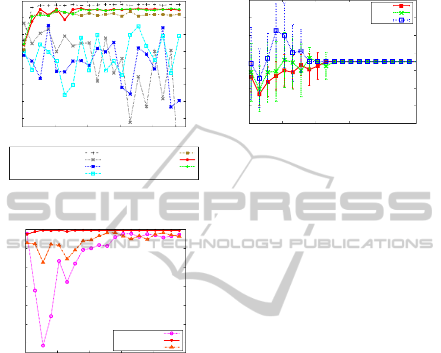
We show the results in Figure 2 and Figure 3. For
comparison, we additionally plotted the averaged ac-
cumulated reward of Sarsa(λ) for the problem with
no delay, that should be regarded as the ideal accu-
racy. In Figure 2, we observe that both MBS+R-max
ICAART 2012 - International Conference on Agents and Artificial Intelligence
582
-140
-120
-100
-80
-60
-40
-20
0
0 20 40 60 80 100
Average reward
Number of episodes
Sarsa(λ) with no delay
Sarsa(λ)
dSARSA(λ) (α=1.0)
dSARSA(λ) (α=0.1)
MBS+R-max
dSARSA(λ)
k
(k=5)
dSARSA(λ)
X
(k
max
=15)
Figure 2: Comparison of Sarsa(λ) with no delay (for refer-
ence), Sarsa(λ), dSARSA(λ), MBS+R-max, dSARSA(λ)
k
,
and dSARSA(λ)
X
, on W-maze.
-1200
-1000
-800
-600
-400
-200
0
0 20 40 60 80 100
Average reward
Number of episodes
dSARSA(λ)
k
(k=4)
dSARSA(λ)
k
(k=5)
dSARSA(λ)
k
(k=6)
Figure 3: dSARSA(λ)
k
for k = 5 (true delay), compared
with k = 4 and 6 (wrong delays), on W-maze.
and dSARSA(λ)
k
given the real delay (k = 5) per-
formed as good as the ideal, Sarsa(λ) with no delay,
while dSARSA(λ) did not. It implies that the predic-
tion in dSARSA(λ)
k
is indeed effective to accelerate
the learning.
Next, we verified the performance of
dSARSA(λ)
k
with varying k. For the same problem,
we executed dSARSA(λ)
k
with k = 4, 5, and 6,
as shown in Figure 3. It is clear that dSARSA(λ)
k
with wrong value (k 6= 5) converges very slowly,
compared to the one with true value k = 5.
Let us turn our attentions to dSARSA(λ)
X
. Fig-
ure 2 shows that dSARSA(λ)
X
learns as quickly
as dSARSA(λ)
k
with true value k = 5, although
dSARSA(λ)
X
does not know the true value. We then
examine how the parameter k
max
affects to the per-
formance of dSARSA(λ)
X
. Figure 4 shows the aver-
age and standard deviation of the predicted delay by
-2
0
2
4
6
8
10
12
0 20 40 60 80 100
Predicted delay
Number of steps
k
max
=5
k
max
=10
k
max
=15
Figure 4: predicted delay by dSARSA(λ)
X
with varying
k
max
on W-maze. We plotted the average and standard de-
viation for every 5 steps.
dSARSA(λ)
X
with k
max
∈ {5, 10, 15}, for 10 times.
X-axis is the number of steps which each algorithm
runs. We see that for any upper bound k
max
= 5, 10,
and 15, predicted delay value converses to the true
value k = 5 before 60 steps. Recall that in Figure 2,
dSARSA(λ)
X
with k
max
= 15 received the reward -
51.3 on average at the first episode. It means that
at the first episode, it consumed 51.3 steps on aver-
age. Moreover, we verified that at the first episode,
dSARSA(λ)
X
consumed 43.7 steps for k
max
= 10,
and 52.0 steps for k
max
= 5 on average, although we
omitted to draw them in the graph. These results im-
ply that the estimation of the true delay finished be-
fore the first episode ends, for any of k
max
= 5, 10,
and 15.
5.1.2 Noisy Environment
We also tried the same problem in noisy environment.
Here, each action succeeds with probability of 0.7,
and otherwise, one of the other three directions is ran-
domly chosen with probability 0.1 for each. In such a
noisy environment, it should be difficult to keep stay-
ing in the same state, so that we cannot apply the naive
algorithm mentioned above.
We determined the meta parameters of learning as
follows. Learning rate α = 0.1, the discount factor γ =
0.5, trace-decay parameter λ = 0.5 for all Sarsa(λ),
dSARSA(λ), dSARSA(λ)
k
and dSARSA(λ)
X
. Ad-
ditionally for dSARSA(λ), we also executed it with
learning rate α = 0.01. As action policies, we chose
the greedy action selection for all algorithms. For
MBS+R-max, we set T = 10 and K
1
= 10. The de-
lay k = 5 and k
max
= 5 for dSARSA(λ)
X
.
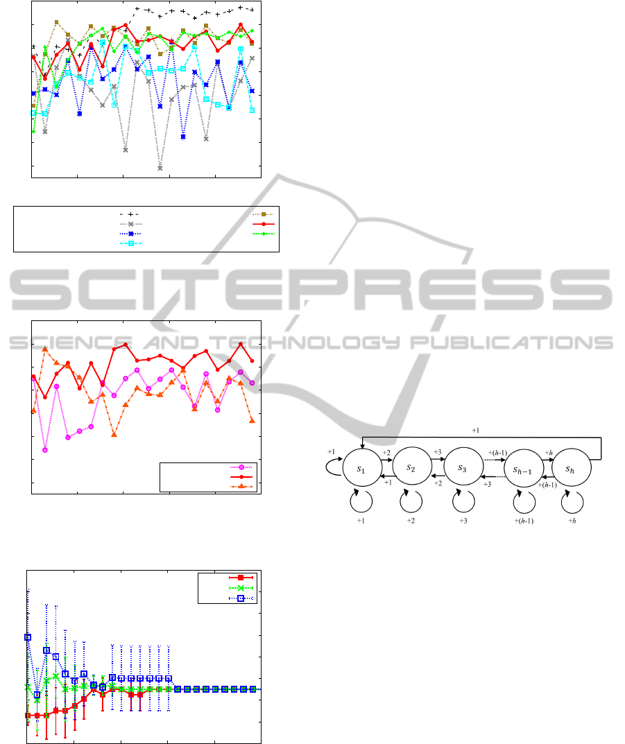
Figure 5, Figure 6, and Figure 7 show the results
in noisy environments, each of which corresponds to
Figure 2, Figure 3, and Figure 4 in noiseless environ-
ment, respectively. We can verify that the problem is
PREDICTION FOR CONTROL DELAY ON REINFORCEMENT LEARNING
583
-140
-120
-100
-80
-60
-40
-20
0
0 20 40 60 80 100
Average reward
Number of episodes
Sarsa(λ) with no delay
Sarsa(λ)
dSARSA(λ) (α=0.1)
dSARSA(λ) (α=0.01)
MBS+R-max
dSARSA(λ)
k
(k=5)
dSARSA(λ)
X
(k
max
=15)
Figure 5: Comparison of Sarsa(λ) with no delay (for refer-
ence), Sarsa(λ), dSARSA(λ), MBS+R-max, dSARSA(λ)
k
,
and dSARSA(λ)
X
, on Noisy W-maze.
-140
-120
-100
-80
-60
-40
-20
0
0 20 40 60 80 100
Average reward
Number of episodes
dSARSA(λ)
k
(k=4)
dSARSA(λ)
k
(k=5)
dSARSA(λ)
k
(k=6)
Figure 6: dSARSA(λ)
k
for k = 5 (true delay), compared
with k = 4 and 6 (wrong delays), on Noisy W-maze.
0
2
4
6
8
10
12
14
16
0 50 100 150 200 250
Predicted delay
Number of steps
k
max
=5
k
max
=10
k
max
=15
Figure 7: Predicted delay by dSARSA(λ)
X
with varying
k
max
on Noisy W-maze. We plottedthe average and standard
deviation for every 10 steps.
indeed more difficult than the problem with no delay;
the learning is slow and the total reward is smaller
than Sarsa(λ) with no delay, because of the strong
noise. However, if we turn our attention to the al-
gorithms for known delay, dSARSA(λ)
k
is more ef-
ficient than the other algorithms. We also see that
dSARSA(λ)
X
performs as good as dSARSA(λ)
k
, al-
though the former does not know the delay while the
latter knows it. Moreover, although the problem can-
not be solved by the naive algorithm , dSARSA(λ)
X
succeeded to estimate the delay accurately; estimation
finished before the first three episodes end.
5.2 Cliff Edge Problem
We propose a new problem, named cliff edge problem
which is illustrated in Figure 8. Imagine the situation
that an agent approaches to the cliff edge at the right
ende. The nearer to the cliff edge the agent stands,
the higher rewards it gets. However, it approaches too
nearly, it falls down. Formally, the agent can observe
its own position as state s
1
, . . . , s
h
. Started from the
initial position s
1
, the agent selects an action among
LEFT, STAY, and RIGHT at each step, and the next
state is decided deterministically. The agent gets a
reward of +i when agent is in state s
i
. However, if the
agent tries to move RIGHT at state s
h
, it returns to the
leftmost (initial) position.
Figure 8: Cliff edge problem: Agent selects a action among
LEFT, STAY, RIGHT at each state in {s
1
, . . . , s
h
}. Agent
get a reward of +i when agent is in state s
i
.
The problem would be easy with no delay under
noiseless environment. However, if we consider the
delay and/or noise, it would be considerably difficult,
since inaccurate observation of the state is fatal to the
agent.
We determined the meta parameters in the same
way as the previous experiment. The learning
rate α = 0.3, the discount factor γ = 0.2, trace-
decay parameter λ = 0.4 for Sarsa(λ), dSARSA(λ),
dSARSA(λ)
k
and dSARSA(λ)
X
. Moreover, we also
examined dSARSA(λ) with the learning rate α =
0.03. We chose the softmax action selection as action
policy for Sarsa(λ), dSARSA(λ)
k
, dSARSA(λ)
X
,
and let the inverse temperature β be 0.2. The delay
k = 5, and the uppper bound of the delay k
max
= 15
for dSARSA(λ)
X
. We executed 3,000 steps from the
initial position as one episode. We repeated it for 10
ICAART 2012 - International Conference on Agents and Artificial Intelligence
584
times and calculated the average of reward at each
step.
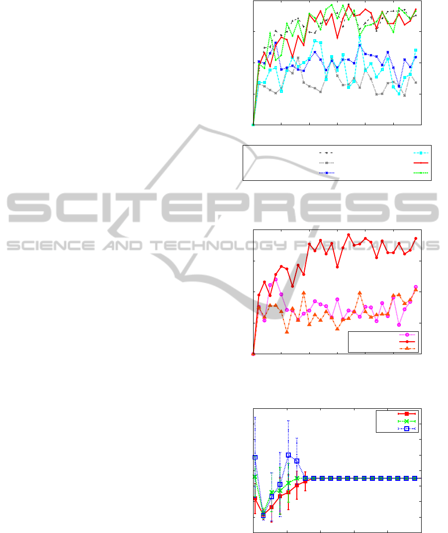
5.2.1 Noiseless Environment
The results in noiseless environment are shown in
Figure 9 and Figure 10. For comparison, we addi-
tionally plotted the averaged reward of Sarsa(λ) for
the problem with no delay. Furthermore, we show
the average and standard deviation of 10 times for
the prediction of state by dSARSA(λ)
X
with k
max
∈
{5, 10, 15} in Figure 11.
These results have almost the same tendency to the
previous experiments on “W-maze”. If the delay k is
known correctly, dSARSA(λ)
k
performs better than
the other methods. For unknown k, dSARSA(λ)
X
converges to the real value quickly.
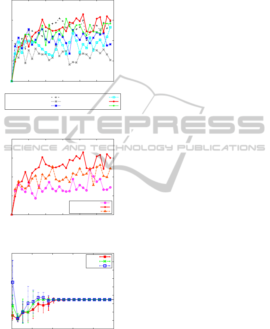
5.2.2 Noisy Environment
We also tried the same problem “cliff edge” in noisy
environment, where the agent moves to the desired
direction with probability 0.9, but moves randomly to
one of the other two directions with probability 0.05
for each. We chose the meta parameters as follows,
based on prior experiments. The learning rate α =
0.05, the discount factor γ = 0.2, trace-decay param-
eter λ = 0.4 for Sarsa(λ), dSARSA(λ), dSARSA(λ)
k
and dSARSA(λ)
X
. Additionally for dSARSA(λ), we
also execute it with the learning rate α = 0.005. As
action policies, we chose the softmax action selection
for Sarsa(λ), dSARSA(λ)
k
, and dSARSA(λ)
X
, and
let the inverse temperature β be 0.5. The delay k = 5
and the upper bound k
max
= 15 for dSARSA(λ)
X
.
Figure 12, Figure 13, and Figure 14 in noisy environ-
ments corresponds to Figure 9, Figure 10, and Fig-
ure 11 in noiseless environments, respectively.
Because of the noise, the learning task became
significantly difficult. However, efficiency of pro-
posed algorithms is as same as the Sarsa(λ) with no
delay, and convergence of prediction of state is also
fast.
6 CONCLUSIONS
In this paper, we dealt with the reinforcement learn-
ing for environments with control delay. We pro-
posed dSARSA(λ)
k
that improved dSARSA(λ) by
predicting current states, which works for known de-
lay. We verified that dSARSA(λ)
k
performs as ac-
curate as MBS+R-max, which is one of model-based
learning algorithms requiring much more computa-
tion resources, while dSARSA(λ) did not work well.
0
5
10
15
20
0 500 1000 1500 2000 2500 3000
Average reward
Number of steps
Sarsa(λ) with no delay
Sarsa(λ)
dSARSA(λ) (α=0.3)
dSARSA(λ) (α=0.03)
dSARSA(λ)
k
(k=5)
dSARSA(λ)
X
(k
max
=15)
Figure 9: Comparison of Sarsa(λ) with no delay (for
reference), Sarsa(λ), dSARSA(λ), dSARSA(λ)
k
, and
dSARSA(λ)
X
, on Cliff edge problem.
0
5
10
15
20
0 500 1000 1500 2000 2500 3000
Average reward
Number of steps
dSARSA(λ)
k
(k=4)
dSARSA(λ)
k
(k=5)
dSARSA(λ)
k
(k=6)
Figure 10: dSARSA(λ)
k
for k = 5 (true delay), compared
with k = 4 and 6 (wrong delays), on Cliff edge problem.
-2
0
2
4
6
8
10
12
14
0 20 40 60 80 100
Predicted delay
Number of steps
k
max
=5
k
max
=10
k
max
=15
Figure 11: Predicted delay by dSARSA(λ)
X
with varying
k
max
on Cliff edge problem. We plotted the average and
standard deviation for every 5 steps.
For the case that the delay is unknown,
we proposed dSARSA(λ)
X
, that combines sev-
PREDICTION FOR CONTROL DELAY ON REINFORCEMENT LEARNING
585
0
5
10
15
20
0 500 1000 1500 2000 2500 3000
Average reward
Number of steps
Sarsa(λ) with no delay
Sarsa(λ)
dSARSA(λ) (α=0.05)
dSARSA(λ) (α=0.005)
dSARSA(λ)
k
(k=5)
dSARSA(λ)
X
(k
max
=15)
Figure 12: Comparison of Sarsa(λ) with no delay (for
reference), Sarsa(λ), dSARSA(λ), dSARSA(λ)
k
, and
dSARSA(λ)
X
, on Noisy Cliff edge problem.
0
5
10
15
20
0 500 1000 1500 2000 2500 3000
Average reward
Number of steps
dSARSA(λ)
k
(k=4)
dSARSA(λ)
k
(k=5)
dSARSA(λ)
k
(k=6)
Figure 13: dSARSA(λ)
k
for k = 5 (true delay), compared
with k = 4 and 6 (wrong delays), on Noisy Cliff edge prob-
lem.
-2
0
2
4
6
8
10
12
14
16
0 20 40 60 80 100
Predicted delay
Number of steps
k
max
=5
k
max
=10
k
max
=15
Figure 14: Predicted delay by dSARSA(λ)
X
with varying
k
max
on Noisy Cliff edge problem. We plotted the average
and standard deviation for every 5 steps.
eral dSARSA(λ)
k
’s as slaves. We confirmed that
dSARSA(λ)
X
performs competitively as the algo-
rithms given the real delay.
As future work, we are interested in theoretical
analysis and expanding for continuous states, actions
and time, as well as applications to real environments.
ACKNOWLEDGEMENTS
This work was partially supported by Kakenhi
23300051.
REFERENCES
Abbeel, P., Coates, A., Qugley, M., and Ng, A. Y. (2007).
An application of reinforcement learning to aerobatic
helicopter flight. In In Advances in Neural Informa-
tion Processing Systems 19, pages 1–8.
Brafman, R. I. and Tennenholtz, M. (2003). R-max-a gen-
eral polynomial time algorithm for near-optimal rein-
forcement learning. The Journal of Machine Learning
Research, 3:213–231.
Freund, Y. and Schapire, R. (1997). A desicion-theoretic
generalization of on-line learning and an application
to boosting. volume 55, pages 119–139.
Katsikopoulos, K. and Engelbrecht, S. (2003). Markov de-
cision processes with delays and asynchronous cost
collection. IEEE Transactions on Automatic Control,
48(4):568–574.
Loch, J. and Singh, S. (1998). Using eligibility traces to
find the best memoryless policy in partially observ-
able markov decision processes. In Proceedings of
the 15th International Conference on Machine Learn-
ing (ICML ’98), pages 323–331.
Schuitema, E., Busoniu, L., Babuˇska, R., and Jonker, P.
(2010). Control delay in reinforcement learning for
real-time dynamic systems: a memoryless approach.
In Proceedings of the 2010 IEEE/RSJ International
Conference on Intelligent Robots and Systems, pages
3226–3231.
Sutton, R. S. and Barto, A. G. (1998). Reinforcement Learn-
ing: An Introduction (Adaptive Computation and Ma-
chine Learning). The MIT Press.
Szita, I. and Szepesv´ari, C. (2010). Model-based reinforce-
ment learning with nearly tight exploration complex-
ity bounds. In Proceedings of the 27th International
Conference on Machine Learning (ICML ’10), pages
1031–1038.
Walsh, T. J., Nouri, A., Li, L., and L.Littman, M. (2007).
Planning and learning in environments with delayed
feedback. In Proceedings of the 18th European Con-
ference on Machine Learning (ECML ’07), pages
442–453.
ICAART 2012 - International Conference on Agents and Artificial Intelligence
586
