
SMART INTEGRATION OF ELECTRIC VEHICLES IN AN ENERGY
COMMUNITY
Ebisa Negeri and Nico Baken
Delft University of Technology, Delft, The Netherlands
Keywords:
Smart Grid, Load Balancing, Distributed Generation, Electric Vehicle.
Abstract:
With increasing penetrations of renewable distributed generations (DGs) and electrified vehicles (EVs), the
volatility of the renewable sources and the huge load of the EVs induce tremendous challenges for the power
grid. The two technologies also have considerable synergetic potential to alleviate these challenges if they are
intelligently coordinated. The aim of this paper is to investigate how the (dis)charging of EVs could be intelli-
gently coordinated with the production of the local DGs to reduce the peak load on the power grid. We consider
a neighborhood energy community that is composed of prosumer households. Three EV (dis)charging scenar-
ios are compared: the dumb strategy where all EVs are charged for the next commute as soon as they return
from the previous commute, the centralized (dis)charging strategy where the EVs are managed by a central-
ized scheduling unit, and the distributed (dis)charging strategy where the households autonomously schedule
their EVs while coordination is achieved through providing dynamic pricing based incentives. Our simulation
results show that the distributed and centralized charging strategies can reduce the peak load up to 44.9%
and 75.1%, respectively, compared to the dumb charging strategy. Moreover, the relative performnce of the
algorithms with respect to environmental values.
1 INTRODUCTION
As distributed generations (DGs) are increasingly
penetrating into the lower parts of the power grid,
the end consumers, such as households, are evolv-
ing from passive consumers to active prosumers. Ac-
cording to the EU parliament, all buildings built af-
ter 2019 will have to produce their own energy on
site
1
. Production of own power on site leads to for-
mation of energy communities (Melo and Heinrich,
2011) that could autonomously manage their own re-
sources and locally exchange power with themselves.
On the other hand, the increasing trend in electrifica-
tion of the transportation sector is expected to bring
about massive presence of electrified vehicles (EVs)
in the near future.
Since most of the DGs have intermittent electric-
ity production patterns, their large composition might
lead to unacceptable volatile profiles that disrupt the
grid stability, power quality, and infrastructure con-
straints. Likewise, presence of an EV doubles the
average power demand of a household (Ipakchi and
1
European Parliament, “All New Buildings to be Zero
Energy from 2019,” Committee on Industry, Research and
Energy, Brussels 2009.
Albuyeh, 2009), thus its massive presence imposes
very large load on the grid. On the other hand, the
EVs provide considerable flexibility that could be ex-
ploited to minimize these challenges. Given that EVs
are idle 95% of the time, more than 90% of all ve-
hicles are parked at any given point in time with
more than 25% of them parked at home (Fluhr et al.,
2010), their charging could be conveniently shifted to
periods of surplus local production. Moreover, the
vehicle-to-grid (V2G) technology gives the possibil-
ity of discharging from the EV back to the grid dur-
ing peak demand periods. Thus, by coordinating the
(dis)charging of the EVs with the local production of
DGs, one can reduce the load of the EVs on the grid,
shield the intermittence of the DGs from the grid, and
reduce the carbon footprint of the EVs. Accordingly,
EVs and DGs seem to form a natural combination.
Although there are a few works in the litera-
ture that consider the synergy between the renewable
sources and the EVs ((Markel et al., 2009), (Lund and
Kempton, 2008), (Verzijlbergh et al., 2011)), they fo-
cus on a high-level study of the coordination of fleets
of EVs and large scale renewable sources on large ge-
ographical regions, without considering the local ef-
fects on the grid constraints and the driving behaviors
of the users of the EVs. In this paper, we endeavor
25
Negeri E. and Baken N..
SMART INTEGRATION OF ELECTRIC VEHICLES IN AN ENERGY COMMUNITY.
DOI: 10.5220/0003952400250032
In Proceedings of the 1st International Conference on Smart Grids and Green IT Systems (SMARTGREENS-2012), pages 25-32
ISBN: 978-989-8565-09-9
Copyright
c
2012 SCITEPRESS (Science and Technology Publications, Lda.)

to fill this gap by investigating how the (dis)charging
of EVs can be efficiently coordinated with the local
generation of power from DGs to minimize the peak
load while considering the local grid constraints and
the driving behaviors. We consider a model futuris-
tic residential neighborhoodenergy community that is
described in the next section. We present three differ-
ent EV (dis)charging strategies: a reference dull strat-
egy, a centralized strategy and a distributed strategy.
The relative gain of these strategies are compared.
The remainder of this paper is organized as fol-
lows. The architecture of the energy community is
presented in Section 2. After describing the system
model in Section 3, we go on to present the three co-
ordination strategies in Section 4. In Section 5, we
present and discuss the simulation results, then we fi-
nalize the paper with the concluding remarks in Sec-
tion 6.
2 THE NEIGHBORHOOD
ENERGY COMMUNITY
In our work, we consider a neighborhood energycom-
munity that is connected to a single medium-voltage
to low-voltage (MV/LV) transformer. A simplified di-
agram of such a neighborhood is shown in Figure 1.
The energy community comprises of prosumer house-
holds. The prosumer households can autonomously
manage their own load profile. Each household can
generate, store, import or export power. Power can be
exchanged between the prosumer households in the
community as well as between the energy community
and the MV grid in either direction.
A multi-agent based control is used to coordinate
the households. Each household has a household-
agent that coordinates its resources to optimize
the household consumption. A community-agent
watches over the overall load distribution of the com-
munity and coordinates the household-agents accord-
ingly. In addition, the community-agent manages the
energy exchange with the rest of the grid.
The energy community is assumed to have a smart
grid infrastructure in place. Each agent in the en-
ergy community has an intelligent device that can
exchange information with the other agents across a
communication infrastructure, and process the infor-
mation to make decisions.
3 THE SYSTEM MODEL
In this section, the mathematical model of the energy
Figure 1: A schematic diagram of a neighborhood energy
community.
community is presented. We consider a scheduling
time period τ (24h) that is divided into time steps, i.e.
τ = {1, 2, ..., T}, that have equal duration of ∆ time
units (15 min.).
3.1 Electric Vehicle
To characterize each EV, the parameters of its bat-
tery are important. The battery parameters of interest
for this work are the following: the maximum energy
storage capacity (Φ in kWh), the cycle efficiency (η
in %), the maximum depth of safe discharging to pro-
long battery life (δ
ch
in %), and the maximum level of
safe charging to prolong battery life (δ
dch
%). Assum-
ing a symmetric cycle efficiency, we denote the stor-
age charging efficiency and discharging efficiency by
η
ch
and η
dch
, respectively, where η
ch
= η
dch
=
√
η.
The state of charge (SOC) of the battery at time step i
is denoted by ψ
i
. The amount of electrical power con-
sumed to charge the battery of the EV, and the amount
of electrical power supplied from the battery upon dis-
charging (V2G) in time step i are denoted by X
i
and
Y
i
, respectively. After the EV commutes a distance
of l km, the state of charge of its battery drops by an
amount l×ω, where ω is the average amount of stored
battery energy the EV consumes per unit km travelled
(in kWh/km).
In this work, we focus on the impact of EVs on the
power grid of a residential energy community. Thus,
we consider only the case where the EVs are charged
and discharged (V2G) within the energy community
either at home or at a charging station within the com-
munity. We denote the periods of time the EV stays
within its community and away by τ
h
and τ
−h
, respec-
tively. The usage of EV is subject to the constraints
listed in Eq.1-8. Eq.1 states that the SOC at the end
of a time step j can be obtained from the SOC at the
end of the previous time step i by adding the net rise
in the SOC in time step j. The net rise in the SOC re-
sults from the injected energy via charging (∆η
ch
X
j
),
the supplied energy via discharging (∆η
dch
Y
j
) and the
SMARTGREENS2012-1stInternationalConferenceonSmartGridsandGreenITSystems
26

battery energy used in commuting (π
j
). ∆ is em-
ployed here to convert power into energy. Constraints
2 and 3 represent the maximum and minimum bound-
aries, respectively, on the SOC for safety of the bat-
tery. Constraint 4 says that the battery of the EV can-
not be charging and discharging at the same time. On
the other hand, constraints 6 and 5 enforce the maxi-
mum and minimum charging and discharging rates of
the battery, respectively, where υ
ch
and υ
dch
denote
the maximum charging and discharging rates, respec-
tively, of the charger. Constraint 7 reflects that we are
limiting the (dis)charging of the EVs only to the peri-
ods when they are within their community. Whenever
an EV begins to commute a distance of l km, its bat-
tery level should be large enough to commute the dis-
tance, and yet not fall below the minimum safe SOC
after commuting (constraint 8).
The deriving behavior of the EV user is derived
from a mobility data, as will be described in section
5.
ψ
j
= ψ
i
+ ∆(η
ch
X
j
−η
dch
Y
j
) −π
j
, ∀i, j ∈ τ (1)
ψ
i
≤ δ
ch
Φ, ∀i ∈ τ (2)
ψ
i
≥ δ
dch
Φ, ∀i ∈ τ (3)
X
i
= 0 or Y
i
= 0, ∀i ∈ τ (4)
0 ≤ Y
i
≤ υ
dch
, ∀i ∈τ (5)
0 ≤ X
i
≤ υ
ch
, ∀i ∈ τ (6)
X
i
,Y
i
= 0, ∀i ∈ τ
−h
(7)
ψ
i
≥ δ
dch
Φ+ lw, commute of l km begins at i(8)
3.2 Household Demand and Production
The accumulated power demand of all the appliances
of the household in time step i is denoted by D
i
.
This demand does not include the demand of the EV
owned by the household, because the EV is modeled
separately. We designate the total power production
of all the DGs owned by the household in time step i
by P
i
. In this work, we assume that forecasts of D and
P are available for the entire scheduling period. The
net demand of a household in time step i, denoted by
R
i
, is defined as the difference between the demand
(appliances and EV) and the production of the house-
hold (Eq.9). R
i
is upper bounded by the power capac-
ity of the line connecting the household to the grid,
L
th
(Eq.10).
R
i
= [D
i
+ (X
i
−Y
i
)] −P
i
, ∀i ∈ τ (9)
R
i
≤ L
th
, ∀i ∈ τ (10)
3.3 Transformer
The net power flow through the transformer, that con-
nects the community to the rest of the grid, at any
time step i is equal to the net demand of the commu-
nity, P
net
i
given in Eq.11, and is generally constrained
by the threshold capacity of the transformer (P
th
), as
shown in Eq.12. In our case, we loosen the constraint
in Eq.12 and try to minimize the peak load using dif-
ferent charging strategies. Observing the resulting
peak load helps to suggest the optimal value of the
transformer rating to be installed to support the load
profile in the energy community under consideration.
P
net
i
= (
∑
all houses
R
i
), ∀i ∈τ (11)
P
net
i
≤ P
th
, ∀i ∈ τ (12)
4 THE CHARGING STRATEGIES
In this section, we present three EV charging strate-
gies, namely, the dull strategy, the centralized strat-
egy, and the distributed strategy.
4.1 The Dull Strategy
This strategy represents a reference scenario where
the EVs are charged for their next commute as soon
as they return to the community from their previous
commute. The EVs are charged up to the target bat-
tery level without interruption at the maximum pos-
sible rate. Apparently, this strategy does not possess
any intelligence, hence the name dumb.
4.2 The Centralized Strategy
The centralized charging strategy assumes that the en-
ergy community is composed of prosumers that coop-
erate with each other to achieve communal goals. In
this case, (dis)charging of the EVs are scheduled of-
fline in a centralized way by an intelligent scheduling
unit (ISU) that could be located at the community-
agent. As opposed to the dumb strategy, this strat-
egy allows charging of the EVs with variable charg-
ing rates and with possible interruptions. This strat-
egy finds optimal schedules as a solution to a linear
programming problem that is shown in Eq.13, where
peak denotes the peak value of the net demand of the
energy community (P
net
). Apparently, this strategy
aims at aligning the EVs with the local production to
minimize the peak load on the transformer.
minimize peak (13)
subject to Eq. 1-12
SMARTINTEGRATIONOFELECTRICVEHICLESINANENERGYCOMMUNITY
27

4.3 The Distributed Strategy
This strategy is based on the assumption that each
household tends to selfishly maximize its own ben-
efits. The EVs are autonomously scheduled by their
respective owners. Thus, a coordination mechanism
is required to maximize utilization of the locally
generated power. Our coordination mechanism in-
volves a local electronic energy market (Kok et al.,
2005) within the community where the autonomous
households trade electricity with each other, whereby
the autonomy of the energy community allows the
community-agent to propose local price-vectors to
achieve desirable communal goals. The community-
agent provides incentives based on a novel dynamic
pricing model that aims at motivating the community
members to shift their demands to lower the peak load
on the transformer.
4.3.1 The Cost
To handle the power import and export of each house-
hold, the dynamic pricing model has two components
for each time step i: the import tariff (γ
im
i
) and the
export tariff (γ
ex
i
). The cost of the household is mod-
eled in Equation 14 for each time step i, where the
terms (γ
im
i
∗R
i
) and (γ
ex
i
∗R
i
) represent the monetary
cost and benefit, respectively, incurred due to the net
demand of the household.
C
h
i
=
γ
im
i
∗R
i
, if R
i
≥ 0
γ
ex
i
∗R
i
, if R
i
< 0
(14)
4.3.2 The Household Optimization
Each household schedules its EVs to minimize its cost
by solving a linear household optimization problem
that is shown in Equation 15.
minimize
∑
∀i∈τ
C
h
i
(15)
subject to Equations 1-9, 14.
4.3.3 The Dynamic Pricing Model
In order to flatten the overall load distribution of the
neighborhood, the community-agent provides each
household with an incentive that is based on a dy-
namic pricing model. In our dynamic pricing model,
the community-agent proposes a price vector, then
each household-agent schedules the storage unit of
that household and replies with the corresponding
scheduled demand of the household. Based on the
response of all the households, the community-agent
adjusts the price vector using an intelligent learning
mechanism. This is repeated iteratively to obtain a
flattened profile.
In the proposed pricing model, the cost of a unit
power varies from one time step to another depending
on the net demand of the neighborhood energy com-
munity (P
net
). Our pricing model aims at encouraging
the households to shift their scheduled demands away
from the peak periods of the overall scheduled de-
mand of the neighborhood. The optimal tariff for each
time step is determined iteratively. At the (j + 1)
th
it-
eration cycle, the tariff for the i
th
time step is obtained
by adjusting the corresponding tariff in the previous
iteration cycle j using an incremental factor (γ×ξ
j,i
):
θ
j+1,i
= θ
j,i
(1 + γ×ξ
j,i
) (16)
The incremental factor is composed of two terms:
the learning factor (γ) and the deviation factor (ξ
j,i
).
The learning factor is a constant (0 < γ ≤1) that deter-
mines to which extent the deviation factor overrides
the old price vector. The deviation factor captures the
variation of P
net
from its average value. Let P
net
i
be
the net demand of the energy community in the i
th
time step for the j
th
iteration cycle. Let mean be the
average of the net demand:
mean =
1
T
T
∑
i=1
P
net
i
The deviation factor, ξ
j,i
, is given by
ξ
j,i
= sign×
(P
net
i
−mean)
2
∑
T
i=1
(P
net
i
−mean)
2
(17)
where the sign determines whether the incremental
value should be positive or negative. If P
net
i
> mean,
then we add a positive incremental value to the tariff
to reduce consumption in this time step: sign = 1. If
P
net
i
< mean, then we substract an incremental value
from the tariff to increase consumption in this time
step: sign = −1. Clearly, ξ
j,i
reflects the effect of
the offset of the demand from the mean value on the
price vector. The pricing model increases tariff on
the time steps where the overall scheduled demand of
the neighborhood community (P
net
) is above the aver-
age, and reduces tariff when P
net
is below the average,
thereby providing incentives to the households to flat-
ten the overall scheduled neighborhood demand.
The power feed-in tariffs are obtained by sub-
stracting the transport part of the import tariffs as sug-
gested in (Houwing et al., 2011). Consequently,
λ
j
= θ
j
−θ
tr
, ∀j ∈τ (18)
where θ
tr
is the transport part of the import tariff θ
j
.
4.3.4 The Distributed Algorithm
Our proposed distributed algorithm comprises of two
types of algorithms. The first type of algorithm (Al-
gorithm 1) is implemented at the community-agent
SMARTGREENS2012-1stInternationalConferenceonSmartGridsandGreenITSystems
28

while the other (Algorithm 2) is implemented at each
household-agent. These algorithms iteratively solve
the household optimization problems by exchanging
information. The iteration cycles continue for a fixed
number of iterations maxIteration, while searching
for an optimal price vector that yields the smallest
peak value for the overall net demand of the neigh-
borhood energy community (P
net
).
The block diagram describing the execution of the
algorithms is shown in Figure 2. At each iteration
step, the community-agent sends the recent tariff in-
formation to each household-agent. Then, it receives
the scheduled demand of the households subject to
the corresponding tariff. Afterwards, it computes the
tariffs for the next iteration cycle based on the overall
scheduled demand of the community (P
net
). On the
other hand, each household-agent in each iteration cy-
cle solves its household optimization problem using
the tariff information received from the community-
agent. It then sends the updated scheduled demand of
the household (R) to the community-agent.
Figure 2: Block diagram of the distributed charging strat-
egy.
Algorithm 1: Executed at neighborhood agent.
1: Initialize θ and λ, counter = 0
2: repeat
3: send θ and λ to each household
4: Receive R from each household
5: Update P
net
using Eq. 11
6: Update θ and λ using using Eq.16 and Eq.18.
7: increment counter by 1
8: until counter ≤ maxIteration
9: send a “DONE” message to each household
Algorithm 2: Executed at each household.
1: repeat
2: receive θ and λ from the neighborhood agent
3: solve the household optimization problem in Eq.15
4: update R according to the solution
5: send R to the neighborhood agent
6: until a “DONE” message is received from the neigh-
borhood agent
Solving the optimization problems is initiated at
the community-agent (Algorithm 1). The algorithm
starts by initializing the tariffs (θ and λ) to flat price
vectors and the iteration cycle counter (counter) to
zero in line 1. In each iteration cycle, lines 3-7 are
executed. In line 3, the recent tariff information is
sent to each household-agent which will be used by
the household-agent to solve the household optimiza-
tion problem in the current iteration cycle. It then re-
ceives from each household-agent its scheduled de-
mand (R) resulting from the solution of the house-
hold optimization problem in the current iteration cy-
cle (line 4). After computing the overall net demand
of the neighborhood P
net
in line 5, the tariffs used in
the next iteration cycle are updated accordingly (line
6). The iteration continues until the iteration count is
equal to maxIteration. The algorithm finalizes the op-
timization process by sending the “DONE” message
to all the household-agents (line 9). The optimal tariff
is chosen by selecting tariff vectors that yielded the
lowest peak value of P
net
.
The algorithm at each household-agent (2) itera-
tively solves the household optimization problem. In
each iteration cycle, the algorithm receives the up-
to-date tariff information from the community-agent
(line 2), solves its optimization problem using the new
tariffs (line 3), updates the scheduled demand of the
household according to the solution (line 4) and sends
it back to the neighborhood-agent (line 5). The itera-
tion continues until a “DONE” message is received.
5 SIMULATION
5.1 Simulation Data
The data for the demand and electricity production
of a household are acquired from Alliander
2
. The
DGs of the household are a PV panel and a micro-
CHP. The data were obtained by field measurements
that were taken every 15 minutes for a duration of 24
hours using smart meters installed at the households.
The micro-CHP generation is constant (1 kW) over
each period of operation, and the data specifies the
start time and end time of each period of its opera-
tion. To make alternative profiles for each household,
we randomized the values according to a normal dis-
tribution around the measured values. A sample of the
daily production and demand profile of a household is
shown in Fig. 3.
The driving behavior of the EV users are con-
structed based on the data from the 2009 mobility re-
2
Alliander is the largest electricity distribution network
operator company in the Netherlands owning 40% of the
distribution networks.
SMARTINTEGRATIONOFELECTRICVEHICLESINANENERGYCOMMUNITY
29
10 20 30 40 50 60 70 80 90
0
0.2
0.4
0.6
0.8
1
1.2
Time Steps
Power (kW)
demand
micro−CHP
PV panel
Figure 3: A sample household demand and production pro-
files.
10 20 30 40 50 60 70 80 90 100
0
0.1
0.2
0.3
0.4
0.5
0.6
0.7
0.8
0.9
1
distance (km)
cummulative probability
Figure 4: Distribution of the distance travelled per day per
car driver.
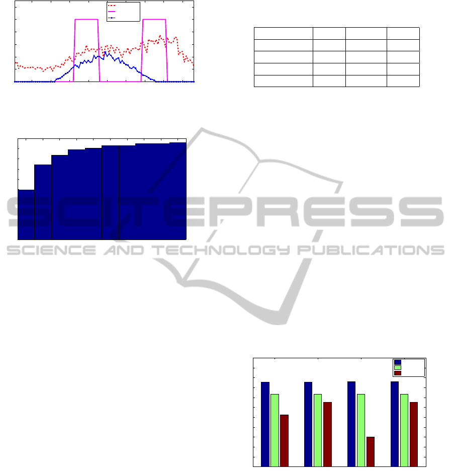
search of the Netherlands (MON, 2009). Fig. 4 shows
the distribution of the distance traveled per car driver
per day as extracted from the data. The commute
distances used in the simulations are generated us-
ing a function with exponential distribution that best
fits the data. For each commute, the departure and
arrival time from/at home are generated using Gaus-
sian functions that best approximate the data obtained
from (MON, 2009).
In our simulations, we involve three types of elec-
tric cars whose technical specifications and market
share are specified in (Knapen et al., 2011), as pre-
sented in Table 1. The composition of the EVs in
the energy community is in line with the market share
values in Table 1. The values of the cycle efficiency
of the batteries, the safe charging level and the safe
discharging level are adopted from (Lombardi et al.,
2009), with the values η = 95%, δ
ch
= 90%, and
δ
dch
= 30%. We conducted our simulations with com-
munity size, N = 50 households, with a conservative
assumption that each household owns one EV. The
average number of cars per household is about 1.6
according to (MON, 2009), thus our assumption of
one EV per household represents roughly 62% pene-
tration of the EVs. We assume that each household
is connected to the grid with a standard connection of
230V and 40A (the case in The Netherlands) resulting
in a line limit of L
th
= 9.2 kW.
Table 1: Technical characteristics for vehicles in specific
categories, and their market share (Knapen et al., 2011).
EV category small medium large
Market share 0.496 0.364 0.140
Φ [kWh] 10 20 35
Range [km] 100 130 180
ω [kWh/km] 0.1 0.15 0.19
5.2 Simulation Results
We present different cases that compose our simu-
lation scenarios. We consider two types of charg-
ers: slow charger (υ
ch
=3.3 KVA) and fast charger
(υ
ch
=7.2 kVA), that are compatible with the Flem-
ish grid (Knapen et al., 2011). Moreover, we con-
sider two cases: chargingwith V2G and without V2G.
While the first case allows feeding from the EV bat-
tery back to the grid, the later does not allow it. We as-
sume that the rate of V2G discharging is constrained
by the same threshold value, i.e., υ
dch
= υ
ch
. In ad-
dition, two cases are considered concerning the target
battery level at the start time of each commute. In the
first case we assume that the target battery level is just
sufficient to support the commute (Eq. 8), whereas in
the second case the target battery level is the maxi-
mum safe charging level of the battery (90% of Φ).
Combining these cases, we present eight simulation
scenarios to compare the performance of our charg-
ing strategies.
slow, with V2G slow, w/o V2G fast, with V2G fast, w/o V2G
0
5
10
15
20
25
30
35
40
45
50
55
community peak demand (kW)
dumb
distributed
centralized
24.6
14.6
65
14.7
24
14
38.8
14.2
Figure 5: Comparison of the algorithms based on the peak
demand of the community (target battery level is commute
energy).
For the case when the target battery level at the
start of each commute is the energy required for the
commute, the relative performance of the charging
strategies under four different scenarios are presented
in Fig.5. The numbers on the top of the bars represent-
ing the distributed and the centralized charging strate-
gies denote the percentage reduction in the peak load
as compared to the dumb charging strategy. As can
be observed from the figure, the distributed charging
SMARTGREENS2012-1stInternationalConferenceonSmartGridsandGreenITSystems
30

slow, with V2G slow, w/o V2G fast, with V2G fast, w/o V2G
0
20
40
60
80
100
120
140
160
community peak demand (kW)
dumb
distributed
centralized
26.6
59.7
11.8
59.7
44.9
75.1
12
74.2
Figure 6: Comparison of the charging strategies based on
the peak demand of the community (target battery level is
90% of the battery capacity).
strategy yields a reduction in the peak load by around
14% in all the four scenarios, which averageto 14.4%.
On the other hand, the centralized charging strategy
reduces the peak by as large as 65%, with average im-
provement of 38.1%.
Figure 6 depicts the relative performance of the
charging strategies when the target battery level at the
start of each commute is 90% of the battery capac-
ity. In this scenario, the distributed charging strategy
achieves an average peak reduction of 23.9%, where
its largest reduction is as high as 44.9%. Whereas
the centralized charging strategy obtains 67.2%, with
75.1% largest improvement.
All the simulation results reveal that the dumb
charging strategy results in large peak demands which
arise from the simultaneous charging of EVs right af-
ter they arrive at home. In the contrary, the central-
ized charging strategy has effectively revealed the po-
tential of the synergy between the EVs and the lo-
cal production to reduce the peak load by exploiting
the flexibility of the EVs. However, the centralized
charging strategy represents a situation where all the
households are cooperative to reduce the peak load
and all the EVs are managed by a centralized unit,
which might contradict the tendency of the house-
holds to autonomously manage their own EVs. On
the other hand, the distributed charging strategy de-
livers 11% to 44.9% reduction in peak demand over
the dumb charging strategy while respecting the au-
tonomy of the households to manage their own EVs.
The strength of the distributed strategy lies in the dy-
namic pricing model that is used as incentive to co-
ordinate the autonomous households that tend to self-
ishly minimize their cost. These improvements are
vital because they reduce the load on the transformer
connecting the energy community with the remain-
ing power grid. The reduction in the peak values has
the advantage of increasing the lifetime of the trans-
former as well as minimizing the need for installing
large capacity transformer.
6 CONCLUSIONS
In an energy community composed of prosumer
households that own EV, the aggregate load profile
might become highly volatile due to the intermittence
of the distributed generations as well the load of the
EVs, which could lead to a large peak load that might
exceed the capacity of the transformer. We have pro-
posed a centralized and a distributed EV charging
strategies that try to minimize the peak load in such
scenario by exploiting the synergy between the lo-
cal distributed generations and the flexibility of the
EVs. Our centralized charging strategy schedules the
(dis)charging of the EVs at a centralized unit assum-
ing that all the prosumers in the energy community
cooperate with each other to minimize the peak de-
mand. Our distributed charging strategy, however,
assumes that the prosumer households autonomously
manage their EVs and tend to selfishly minimize their
cost. Our distributed strategy coordinates the house-
holds to minimize the peak demand by providing in-
centives based on our novel dynamic pricing model.
In addition to presenting a detailed model of the sys-
tem taking into consideration the local constraints, we
have derived the driving behaviors of the EV users
from a realistic mobility data. Based on our simula-
tion results, we have shown that our centralized and
distributed charging strategies can reduce the peak by
as large as 75.1% and 44.9%, respectively, compared
to a reference dumb charging strategy. Therefore, our
proposed strategies can help to reduce the load on the
transformer connecting the energy community to the
rest of the grid, and also minimizes the need for up-
grading the capacity of the transformer.
REFERENCES
Fluhr, J., Ahlert, K., and Weinhardt, C. (2010). A stochastic
model for simulating the availability of electric vehi-
cles for services to the power grid. In 43rd HICSS,
2010, pages 1–10. IEEE.
Houwing, M., Negenborn, R., and De Schutter, B. (2011).
Demand response with micro-chp systems. Proceed-
ings of the IEEE, 99(1):200–213.
Ipakchi, A. and Albuyeh, F. (2009). Grid of the future.
Power and Energy Magazine, IEEE, 7(2):52–62.
Knapen, L., Kochan, B., Bellemans, T., Janssens, D., and
Wets, G. (2011). Activity based models for coun-
trywide electric vehicle power demand calculation.
SGMS.
Kok, J., Warmer, C., and Kamphuis, I. (2005). Power-
matcher: multiagent control in the electricity infras-
tructure. In Proceedings of the fourth international
joint conference on Autonomous agents and multia-
gent systems, pages 75–82. ACM.
SMARTINTEGRATIONOFELECTRICVEHICLESINANENERGYCOMMUNITY
31

Lombardi, P., Vasquez, P., and Styczynski, Z. (2009). Plug-
in electric vehicles as storage devices within an au-
tonomous power system. optimization issue. In Pow-
erTech, 2009 IEEE Bucharest, pages 1–7. IEEE.
Lund, H. and Kempton, W. (2008). Integration of renew-
able energy into the transport and electricity sectors
through v2g. Energy Policy, 36(9):3578–3587.
Markel, T., Kuss, M., and Denholm, P. (2009). Communi-
cation and control of electric drive vehicles supporting
renewables. In VPPC’09. IEEE, pages 27–34. IEEE.
Melo, H. and Heinrich, C. (2011). Energy balance in a re-
newable energy community. IEEE EEEIC.
MON (2009). Mobility research of the netherlands 2009
(mobilitietsonderzoek nederland (mon) 2009). avail-
able: http://rijkswaterstaat.nl/.
Verzijlbergh, R., Ilic, M., and Lukszo, Z. (2011). The role
of electric vehicles on a green island. In NAPS, 2011,
pages 1–7. IEEE.
SMARTGREENS2012-1stInternationalConferenceonSmartGridsandGreenITSystems
32
