
Multivariable Discrete Time Repetitive Control System
Hammoud Saari
1
and Bernard Caron
2
1
SETRAM, Ecole Nationale Supérieure Maritime, Bou Ismail, Algeria
2
SYMME, Université de Savoie, Annecy le Vieux, France
Keywords: Repetitive Control, Multivariable Systems, Invertible Systems, Non Invertible Systems, Tracking.
Abstract: This paper deals with an iterative learning control law for multivariable systems. The desired inputs are
supposed to be known and periodic. The principle of the control is to make outputs as close as possible to
desired inputs at each new period. After the design of multivariable repetitive controller, we give the
stability condition of the algorithm and some simulation results.
1 INTRODUCTION
The theory of the modern control was successfully
used in the control of several industrial processes.
There are at the moment several analytical methods
for the choice of the controller that permit to obtain
an asymptotic stability and an acceptable static error,
but few of them specify the transient response of the
system. This limitation motivated the researchers to
develop a new concept of control for the systems
that repeat the same operation, known under the
name of iterative learning control either repetitive
control. The objective of such control is to improve
the performances to every new period (Figure 1).
Number of period
0 1 2 3
repetitive input
Output
Figure 1: Example of periodic output.
Typical examples are industrial robots, which
most of their tasks are of this kind; e.g. pick and
place, painting, etc. Other examples are control of
numerical control machines, hard-disc drive or many
mechanical systems having revolving mechanisms
inside.
Several researchers were interested in this type
of control law (Arimoto et al. (1984), Sugie and Ono
(1991), Moore et al. (1992), Xu and Tan (2003),
Ahn et al. (2007) and Saari et al. (2010)). Most of
their works were focused on the problem of the
control in the multivariable case. They approached
this problem by an analysis in the state space. The
criticism made to this analysis is that it did not take
into account the dynamics of the process to be
controlled in the convergence condition of this
algorithm (Curtelin et al. (1993)). The problem was
resolved in the case of Single-Input Single-Output
(SISO) systems by making an analysis by transfer
function (Saari et al. (2010)). By respecting the
convergence condition, the error goes to zero after
an infinite number of periods. This induces the
inversion of the process. The problem of non
minimum phase process appears. This kind of
problem was resolved by introducing the approached
inverse of the process in the repetitive filter
(Tomizuka et al. (1988) and Saari et al. (1994a,
1994b, 1996, 2010)).
In this paper, we are going to generalize the
solution found for SISO systems to a Multi-Inputs
Multi-Outputs (MIMO) system by using the notion
of transfer matrix.
2 PROBLEM FORMULATION
The principle of repetitive control is presented by
Figure 2, where, G is the transfer matrix of the
process supposed to be stable and where
nnG )dim(
. H is the transfer matrix of the
repetitive filter where
nnH )dim(
. Y
d
is the
vector of periodic reference signal of dimension n. Y
i
105
Saari H. and Caron B..
Multivariable Discrete Time Repetitive Control System.
DOI: 10.5220/0003964501050110
In Proceedings of the 9th International Conference on Informatics in Control, Automation and Robotics (ICINCO-2012), pages 105-110
ISBN: 978-989-8565-21-1
Copyright
c
2012 SCITEPRESS (Science and Technology Publications, Lda.)
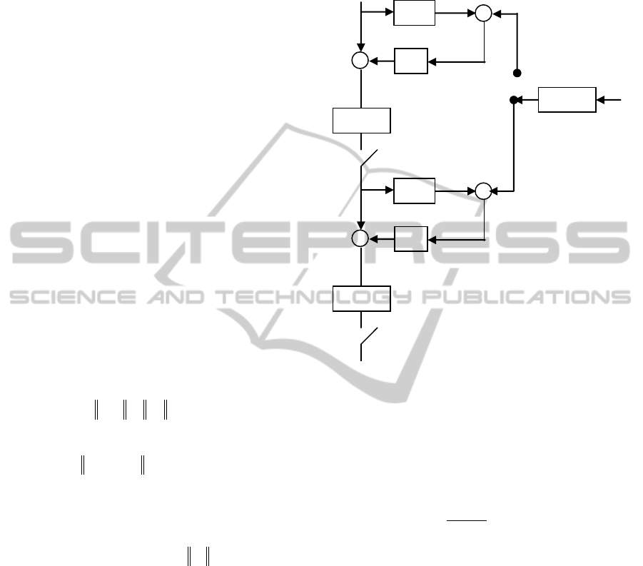
and U
i
are respectively the vectors composed by
output and control signals of the period i. Both
vectors are of dimension n. The memory blocks are
introduced to indicate that the used signals are
memorized in order to be used in the next period.
From Figure 2, one has:
.
11
ii
UGY
(1)
The control algorithm is then given by the
following equation:
,
1 iii
EHUU
(2)
where E
i
is the error vector of dimension n given by:
.
i
d
i
YYE
(3)
By replacing (2) in (1) and taking into account
(3), one obtains:
.
1 ii
EHGIE
(4)
From (4), one can deduce the following theorem
that gives the convergence condition of the repetitive
algorithm.
Theorem 1
The repetitive control algorithm (2) converges and
the error decreases under certain norm;
ii
EE
1
(5)
if and only if:
.1
HGI
(6)
The proof is obvious from (4).
If the convergence condition (6) is verified the
error vector tends towards a null value after an
infinite number of periods (
0lim
i
i
E
), this is
equivalent to
d
YY
and then, the control signal
vector after an infinite number of periods inverts the
process dynamic (
d
YGU
1
) which seems to be
impossible when the plant to be controlled is non
invertible.
However, since Y
d
is an a priori known signal, it
is possible to generate the off-line control signal
vector even if the plant is non invertible (saari et al.
(2010)).
Moore et al. (1992) show that to satisfy the
repetitive control convergence condition, the
repetitive controller H will contain the inverse of the
process. The question is then, what can we do when
the process is non invertible?
In the following, we will examine several
situations of the process to be controlled and
consequently we will give the best choice of
repetitive filter.
Memory
G
H
Memory
U
i
Y
i
- +
E
i
+
+
G
H
Memory
U
i+1
Y
i+1
- +
E
i+1
+
+
Y
d
U
i+2
Figure 2: Scheme of the repetitive control.
3 CASE OF STABLE PROCESS
Let G the discrete stable transfer matrix of the
process given under the form:
,)(
)(
)(
1
1
1
zN
zD
z
zG
d
(7)
where d denotes the delay. D(z
-1
) is the polynomial
denominator of the transfer matrix G, containing the
poles of the process. N(z
-1
) is a matrix which
elements are polynomials.
In this section, we approach the problem of the
choice of repetitive filter in the cases of invertible
and non invertible processes.
3.1 Case of an Invertible Process
A first idea consists in choosing the repetitive filter
H such that it compensates only the delay while
verifying the convergence condition (6).
The simplest expression of H is:
,)(
0
1
HzzH
d
(8)
with H
0
a constant matrix with an appropriate
ICINCO 2012 - 9th International Conference on Informatics in Control, Automation and Robotics
106

dimension.
The drawback of this method is that there is no
method which guides us in the choice of H
0
.
A second idea with the choice of the repetitive
filter H consists in setting the inverse of the transfer
matrix
)(
1
zG
multiplied by a gain kr
such as:
.)()()(
1
111
zNzDzkrzH
d
(9)
Theorem 2
The repetitive control algorithm described by Figure
2, with the repetitive filter (9) for invertible system
(7), converges to zero error vector if and only if:
20 kr
.
Proof:
By examining the convergence condition (6) and by
taking into account (7) and (9), one obtains:
,1
IkrI
(10)
that allows us to write:
,11,,0 kr
and gives us finally:
.20 kr
3.2 Case of Non Invertible Process
The idea in this case, is to put in the repetitive filter
an estimate of the inverse of the process transfer
matrix.
The inverse of the transfer matrix G(z
-1
) appears
under the form:
.)()()(
1
11
1
1
zNzDzzG
d
(11)
One has:
,
)(det
)(
)(
1
1
11
zN
zNadj
zN
(12)
where
)(
1
zNadj
is the adjoint of matrix N(z
-1
) and
)(det
1
zN
is the determinant polynomial of N(z
-1
).
1
1
(
zG
is stable if the roots of
)(det
1
zN
are
located inside the unit circle.
Let us decompose
)(det
1
zN
into a polynomial
containing the roots situated inside the unit circle
)(
1
zN
and another one containing both roots
situated outside of the unit circle and possible delay
)(
1
zN
:
.)()()(det
111
zNzNzN
(13)
We suggest to take the repetitive filter H(z
-1
)
under the form:
.(
)(
)()(
)(
1
1
1
1
zNadj
zNn
zNzDz
krzH
d
(14)
with
.)(max
2
,0
j
eNn
kr is called the repetitive filter gain and
)(zN
is
obtained by replacing every z
-1
in
)(
1
zN
by z.
It is necessary to note that this filter has a strong
similarity with the zero phase tracking controller
(Tomizuka (1987)).
Theorem 3
The repetitive algorithm described by Figure 2, with
the repetitive filter (14) for non invertible system
(7), converges to zero error vector if and only if:
20 kr
.
Proof:
Let us examine the convergence condition (6). By
taking into account (7) and (14) as well as (12), one
obtains:
.1
)()(
1
I
n
zNzN
krI
(15)
One can then write for (15):
,1)()(1max
,0
jj
eNeN
n
kr
that gives us:
,
)()(
2min0
,0
jj
eNeN
n
kr
and finally:
.20 kr
4 CASE OF AN UNSTABLE
PROCESS
In the case of an unstable process, the scheme of the
repetitive control (Figure 2) is modified and
becomes:
Multivariable Discrete Time Repetitive Control System
107

Y
i
Y
d
E
i
K
G
U
i
H
C
i
+
+
+
+
i-1
-
Figure 3: Repetitive control in closed loop configuration.
where K(z
-1
) is a the controller transfer matrix that
stabilizes the loop where
nnK )dim(
. C
i
is the
vector of the output controller’s of dimension n,
i
of dimension n, is an anticipate vector function of
the past error vector and the past control vector and i
indicate the number of period.
Based on this scheme, the control law is then:
.
11
iiii
EKEHUU
(16)
By multiplying the left side of both terms of (16)
by G, one obtains:
,
11
iiii
EKGEHGYY
(17)
and then:
,
11
iiii
EKGEHGEE
(18)
that gives us finally:
.
1
1 ii
EHGIKGIE
(19)
From (19), the repetitive algorithm will converge
to zero error (under certain norm) if:
,1
1
HGIKGI
(20)
and knowing that:
,
BABA
where A and B are two complex matrices.
If one notes:
,
1
KGI
(21)
then the condition (20) becomes:
./1
HGI
(22)
In the case of an invertible process, the repetitive
filter H(z
-1
) was taken like (9) and the convergence
condition of the repetitive algorithm is given by the
following theorem:
Theorem 4
The repetitive algorithm described by Figure 3 with
the repetitive filter given by (9) and for invertible
system (7), converges to zero error vector, if and
only if:
./11/11
kr
(23)
Proof:
By replacing in the convergence condition (22) G
and H by their expressions given respectively by (7)
and (9), one obtains:
,/1
IkrI
(24)
that leads to:
,/11,0
kr
and gives us finally:
./11/11
kr
In the case of a non invertible process, the
repetitive filter H(z
-1
) is taken by the expression
(14). In that case, the convergence condition of the
repetitive algorithm is given by the following
theorem:
Theorem 5
The repetitive algorithm described by Figure 3 for
non invertible system (7) and using the repetitive
filter (14), converges to zero error vector if and only
if:
,
kr
(25)
with:
.
)()(
/11max
,0
jj
eNeN
n
.
)()(
/11min
,0
jj
eNeN
n
Proof:
From the convergence condition (22) and by taking
into account (7), (14) and (12), one obtains:
./1
)()(
1
I
n
zNzN
krI
(26)
With the same approach which was made for
(15), one has:
ICINCO 2012 - 9th International Conference on Informatics in Control, Automation and Robotics
108
,/1)()(1max
,0
jj
eNeN
n
kr
and gives us finally:
.
kr
5 SIMULATION RESULTS
To highlight the theoretical developments made
previously, let us consider the process described by
the following stable transfer matrix:
.
02.01
5.111
3.01
)(
1
1
1
1
1
z
z
z
z
zG
We are in the case of non invertible stable
system (section 3.2).
Let us calculate det(N) that we put under the
shape given by (13):
)2.01()(
)5.11()(
11
111
zzN
zzzN
that allows us to give the following repetitive filter:
,
2.01
)(
2221
1211
1
1
HH
HH
z
kr
zH
with:
2
22
22
21
21
12
11
24.0232.0048.0
24.028.0944.0096.0
24.0592.0396.0072.0
0
zzH
zzzH
zzzH
H
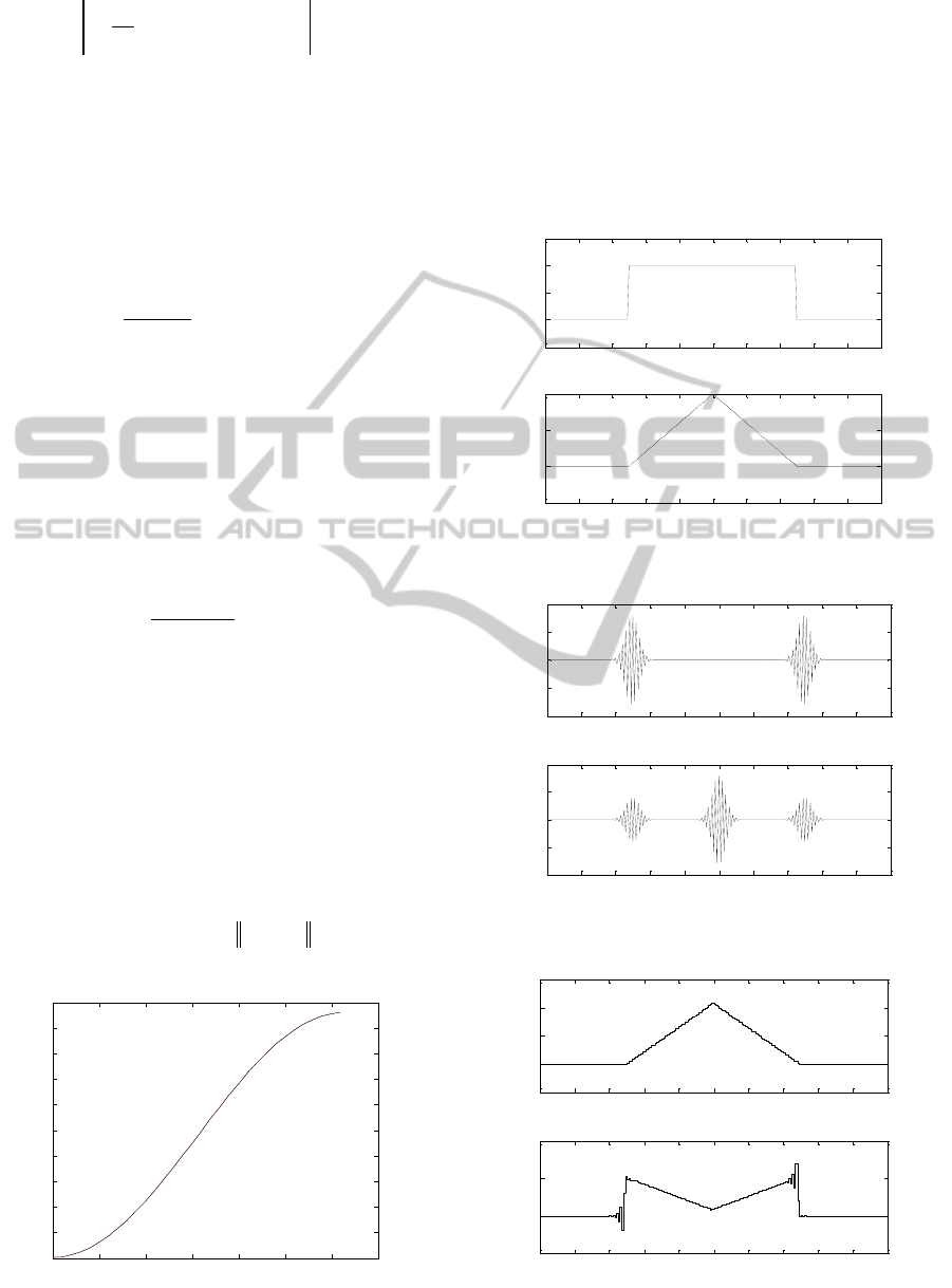
From theorem 3, kr must be included between 0
and 2 so that there is convergence of the repetitive
algorithm. We choose then
1kr
. Figure 4
represents the convergence condition. We can see
that it is respected, seen that
GHI
is lower than
1 like imposed by (6).
0 0.5 1 1.5 2 2.5 3 3.5
0
0.1
0.2
0.3
0.4
0.5
0.6
0.7
0.8
0.9
1
||1-GH||
Pulsation (rad/s)
Figure 4: Convergence condition.
The purpose of this control is to track perfectly
(with zero error) the periodic reference signals given
by Figure 5 and which are represented over a period.
Figure 6 shows the behavior of the tracking error
signals (e
1
and e
2
) at the 30
th
period. One can see that
there are practically zero. We obtain these results
without inverting the process and consequently
without divergence of the control signals u
1
and u
2
,
see Figure 7.
0 20 40 60 80 100 120 140 160 180 200
-0.5
0
0.5
1
1.5
Reference signal Yd1
Time (s)
0 20 40 60 80 100 120 140 160 180 200
-0.5
0
0.5
1
Reference signal Yd2
Time (s)
Figure 5: Reference signals.
0 20 40 60 80 100 120 140 160 180 200
-0.02
-0.01
0
0.01
0.02
Time (s)
Error signal e1
0 20 40 60 80 100 120 140 160 180 200
-4
-2
0
2
4
x 10
-4
Error signal e2
Time (s)
Figure 6: Control signal behavior at the 30
th
period.
0 20 40 60 80 100 120 140 160 180 200
-0.5
0
0.5
1
1.5
Time (s)
Control signal u1
0 20 40 60 80 100 120 140 160 180 200
-0.5
0
0.5
1
Control signal u2
Time (s)
Figure 7: Control signal behavior at the 30
th
period.
Multivariable Discrete Time Repetitive Control System
109

6 CONCLUSIONS
In this paper, we have considered the problem of the
repetitive control in the multivariable case by using
the formalism of the transfer matrix. This formalism
allowed us to consider the processes with stable and
unstable inverse transfer matrix. Moreover, the case
of a closed loop configuration was considered when
the system to be controlled is unstable. This paper
allowed us to generalize the solutions found for
SISO systems. With this algorithm, we obtained
good results (zero error vector) while avoiding the
inversion of the process in order to have no
divergence of the control signals.
REFERENCES
Ahn, H., Moore, K. L. and Chen Y. (2007). Iterative
Learning Control. Robustness and Monotonic
Convergence for Interval Systems, Ed. Springer.
Arimoto, S., Kawamura, S. and Miyazaki, F. (1984).
Bettering Operation of Dynamic System by Learning:
a new control theory for servomechanism or
mechatronics systems, IEEE Proceeding of 23th CDC,
pp. 1064-1069.
Curtelin, G., Saari, H. and Caron. B. (1993). Repetitive
control of continuous systems: Comparative study and
application, Proceeding of IEEE SMC’93, Vol. 5, pp.
229-234.
Moore, K. L., Dehleh, M. and Bhattacharyya, S. P. (1992).
Iterative Learning Control: A Survey and New
Results. Journal of Robotics Systems, 9(5), pp. 563-
594.
Saari, H., Caron, B. and Curtelin, G. (1994a). Perfect
tracking of non minimum phase process. Application
to flexible joint robot, Proceeding of IFAC
SY.RO.CO’94, Vol. 3, pp. 727-733.
Saari, H., Caron, B. and Curtelin, G. (1994b). Optimal
repetitive control, Proceeding of IEEE SMC’94, Vol.
2, pp. 1634-1638.
Saari, H., Tadjine, M. and Caron, B. (1996). Discrete time
repetitive control: Design and robustness analysis,
Proceeding of WAC’96, World Automation Congress,
Intelligent Automation and Control, Vol. 4, pp. 643-
650, TSI Press Series, Albuquerque, N.M.
Saari, H., Caron, B. and Tadjine, M. (2010). On the design
of discrete time repetitive controllers in closed loop
configuration, Automatika, Vol. 51 (4), 333-344.
Sugie. T. and Ono, T. (1991). An iterative control law for
dynamical systems, Automatica, Vol. 27(4), 729-732.
Tomizuka, M. (1987). Zero phase error tracking algorithm
for digital control. ASME Journal of dynamic systems,
measurement and control. Vol. 109, 65-68.
Tomizuka, M., Tsao, T. C. and Chew, K. K. (1988).
Discrete Time Domain Analysis of Repetitive
Controllers, Proceeding of ACC’88, Vol. 2, pp. 860-
866.
Xu, J. and Tan, Y. (2003). Linear and nonlinear iterative
learning control, Ed. Springer.
ICINCO 2012 - 9th International Conference on Informatics in Control, Automation and Robotics
110
