
Reconstruction-based Set-valued Observer
A New Perspective for Fault Detection within Uncertain Systems
Letellier Clément, Chafouk Houcine and Hoblos Ghaleb
Institut de Recherche en Systèmes Electroniques Embarqués, Rouen, France
Keywords: Uncertain Systems, Set-valued Observer, Sensor Reconstruction, Fault Detection.
Abstract: This paper presents an extension of a particular type of observer called the Set-valued Observer; this kind of
observer is very well suited for uncertain fault detection. But some limitations restrict its use. Indeed, all the
sensors are needed to observe the state and as a consequence this method does not allow fault detection
when some sensor information is not available. Other work has focused on the well-known Luenberger
Observer applied to uncertain systems; but once again, this option is limited. Indeed, it is difficult to
converge the algorithm because of the wrapping effect induced by recursivity. Here a new approach is
proposed combining the power of the two algorithms. The Luenberger Observer coupled with the Set-
Valued Observer allows us to reconstruct the states without divergence. This combination is a substantial
contribution for fault detection within uncertain systems.
1 INTRODUCTION
Industrial processes appeared many years ago. They
facilitated the improvement of the quality and
quantity of production. However, these processes are
not infallible. Failures can damage the functional
units of the system such as measurement, action and
control systems which results in a decrease of
productivity.
In order to overcome this problem, monitoring
methods have emerged to detect, isolate and identify
the faults. These methods are known under the
generic name FDI (Fault Detection & Isolation). The
functioning depends on sensor feedback
information. Accompanied with a model, this
information makes it possible to recreate the state
and by extension detect the appearance of faults.
This state reconstruction is of major importance as it
allows us to create virtual sensors which decrease
the system’s cost or the space requirement.
Furthermore, sometimes some of the sensors cannot
be implemented because of measurement
accessibility.
For decades, these systems have brought
substantial advances by estimating the state values
and comparing them to the reference values, making
it possible to obtain residuals and fault indicators.
Many diagnosis methods, such as observers, have
been inspired by this approach. Indeed, a traditional
way to estimate the state relies on observers such as
the Luenberger observer (Luenberger, 1964). An
extension of this method—called the Kalman filter
(Kalman, 1960)—has been developed to deal with
measurement noises. When the latter are white and
Gaussian, the Kalman filter provides the state’s
optimal filter in the sense of minimum variance.
Another approach called “parity space” is based on
the analytical redundancy of state equations (Chow
and Willsky, 1984). The principle is to choose an
orthonormal solution cancelling the observability
matrix in order to obtain fault-sensitive residuals.
Finally, less common methods such as direct filter
synthesis exist. They can be found in two forms:
those based on H∞ robust estimators (Mangoubi,
1998) and those based on the common synthesis of a
dynamic filter and two structure matrices (Henry and
Zolghadri, 2005).
In a general manner all these methods are called
“model-based” or “analytical”. The major problem
of models is they do not represent reality accurately.
Indeed, for instance, it is well known that resistances
in electrical circuits change according to the
surrounding temperature. A fault detection method
relying on such a model will provide false alarms.
From this observation, conventional methods of
diagnosis have been redefined to accommodate the
uncertain framework. Different approaches have
been used to address this problem.
111
Clément L., Houcine C. and Ghaleb H..
Reconstruction-based Set-valued Observer - A New Perspective for Fault Detection within Uncertain Systems.
DOI: 10.5220/0003972301110117
In Proceedings of the 9th International Conference on Informatics in Control, Automation and Robotics (ICINCO-2012), pages 111-117
ISBN: 978-989-8565-21-1
Copyright
c
2012 SCITEPRESS (Science and Technology Publications, Lda.)

First, the active approach attempts to cancel the
uncertainties to overcome their effect at the fault
detection step. Residuals are calculated to be
insensitive to uncertainties while being sensitive to
faults. Several approaches have been developed in
this direction in recent years: the unknown input
observer, the eigenstructure assignment (Chen and
Patton, 1999) and structured parity equations
(Gertler, 1998).
Secondly, the passive approach (Puig et al.,
2002) is based on the propagation of uncertainties in
the estimated values to obtain the enclosures in
which all possible trajectories are included. A fault
is detected when the measurement goes beyond the
enclosure.
Uncertainty modeling is not straightforward. The
primary idea was to model uncertainties in a
statistical manner using confidence intervals. Later,
interval analysis allowed a natural modeling of
uncertainties (Jaulin et al., 2001). In the literature,
interval analysis can be found under the names “set-
membership approach” or “bounding approach”.
Taking the uncertainties into account brings a
new dimension to the diagnosis but is not without
drawbacks.
Based on a recursive computation, observers face
the recurrent phenomenon with uncertain systems
called the wrapping effect. To prevent this
phenomenon— causing the exponential expansion of
the bounds of the state—several methods have been
developed. Some methods are more suitable than
others. Among them, there is the parity space
approach using the bounding approach (Ploix and
Adrot, 2006). Other methods based on interval
observers for fault detection have been presented by
Gouzé et al. (Gouzé et al., 2000) and more recently
by Raïssi et al. (Raïssi et al., 2010). The idea of this
method within uncertain systems is to use two
Luenberger-like observers. In this manner, the
bounds of the states are computed separately: one
observer for the upper value and the other one for
the lower value. On the other hand, another
approach based on LPV and qLPV models have
been developed (Darengosse and Chevrel, 2002).
Finally, the last approach is a particular type of
observer developed for set-membership systems.
This prediction–correction-based observer has been
introduced by Shamma et al. (Shamma and Tu,
1995) and more recently, used by Haimovich et al.
and Benothman et al. (Haimovich et al., 2004;
Benothman et al., 2007). Called “Set-Valued
Observer”, this observer overlaps two pieces of
information: one coming from the model and the
other one from the sensor (Letellier et al., 2011).
In this paper, an extension of this observer will
be presented in order to bypass some limitations by
reconstructing the sensor value when the
measurement is not available.
The paper is organized in the following manner.
Section 2 introduces the problem statement. Section
3 presents the background material used in the
proposed algorithm. The main contribution of the
paper is presented in section 4. Section 5 provides a
numerical example and the simulation results.
Finally, section VI draws the conclusion.
2 PROBLEM STATEMENT
Let us consider an uncertain linear system described
by the following discrete-time dynamic equations:
1kkk
kkk
x
Ax Bu
yCxw
+
=+
⎧
⎨
=+
⎩
(1)
where
∈⊆\D
x
n
x is the state vector of the
system, w is the measurement noise,
∈ \
u
n
u
is the
input vector of the system and
∈ \
y
n
y
is the output
vector of the system. A, B, C are respectively the
state, the input and the output matrices and are
considered uncertain. They are modeled by intervals:
[
]
θ
⇔ ()ZZ
with
{
}
|
θ
θ
θ θθθ
=∈ ≤≤\
n
.
In this paper, the Set-Valued Observer is
extended in order to reconstruct the state when the
measurement is not available.
The conventional Set-Valued Observer is defined
as follows:
{
}
{}
()
[]
1-111
1
|
|
p
kkkkk
em
kkkk
pe
kkk
m
kkk
XAx+BuxX
X=Cy y Y
X=X X
Yyw
−−−
−
⎧
=∈
⎪
∈
⎪
⎪
⎨
∩
⎪
⎪
=+
⎪
⎩
(2)
where
p
k
X
,
e
k
X
and
k
X
are respectively the
predicted state set, the estimated state set and the
corrected state set. The matrices A, B, C are bounded
within intervals. The w measurement noise is
bounded within intervals and added to the
y
measurement.
This observer has numerous advantages for
estimating the state within uncertain systems; the
correction step avoids the wrapping effect. The
major limitation of this observer is the estimation
step where the state is deduced from the sensor.
ICINCO2012-9thInternationalConferenceonInformaticsinControl,AutomationandRobotics
112

Indeed, the observation matrix inversion is not
always achievable. Moreover, when measurements
are not available, the states cannot be deduced from
the sensor.
From this observation, we propose an
improvement on the conventional Set-Valued
Observer. The limitations are bypassed by
reconstructing the state from measurements instead
of deducing it directly. Section 4 will introduce the
proposed method.
3 BACKGROUND MATERIAL
3.1 Interval Tools
The central idea of the interval analysis is to replace
real numbers by intervals
[
]
{
}
|=≤≤\
x
xxxxε
;
in this manner, calculation algorithms can be used to
obtain guaranteed numerical results (Jaulin et al.,
2001).
An interval is defined as a connected subset of
\
noted \I . For instance:
[
]
1, 3
and
[
]
,2−∞ −
are
intervals even though the use of bounded intervals is
recommended.
An interval can be defined in two ways: directly
by the bounds
[
]
inf, sup
or by the couple (Midpoint,
Radius).
The operations are redefined: let us consider an
operator
{
}
;;;/∈+−∗D
and
[
]
[
]
,ab
two intervals,
then
[
]
[
]
[
]
[
]
{
}
|,=∈∈DDab xyxayb
.
The width of an interval
[
]
x
is defined by
[
]
wx x x=−
, its midpoint by
[
]
()
/2mid x x x=+
and its
radius by
[
]
()
/2rad x x x=−
.
3.2 Inclusion Functions
Consider
→f:\\
x
n
m
. The range of the function f
over an interval vector
[
]
x
is given by:
[
]
()
(
)
[
]
{}
=∈ff|
x
xx x
(3)
An interval function
[
]
→f:\\II
x
n
m
is an
inclusion function of f if:
[
]
[
]
(
)
[
]
[
]
(
)
∀⊆∈ ,f f\I
x
n
xx
x
(4)
where
[
]
(
)
f
x
denotes the set-theoretical image of
[
]
x
by f.
4 OBSERVER DESIGN
In this section, an observer architecture, to some
extent analogous to that of the Set-Valued Observer,
will be proposed. Actually, this extension combines
the power of both the SVO and the well-known
Luenberger observer.
The idea here is to use the SVO architecture but
instead of deducing the state directly from the
sensor, we propose reconstructing the state from the
sensor. In this manner, we can implement virtual
sensors and we do not have the limitation of the
observation matrix inversion. To do this, the
Luenberger-like estimation equation is used under
observability conditions. As the SVO has a
correction step, the estimation equation will not
suffer from the wrapping effect due to recursivity.
This method involves three steps as for the
conventional SVO:
1) The Prediction of the state set according to the
model and its uncertainties.
2) The Estimation of the state set according to the
uncertain measurements available and the
model.
3) The Correction of the state set by computing
the intersection of both previous sets
In the rest of this paper we will call the proposed
architecture Set-Valued Luenberger Observer
(SVLO) to distinguish it from the conventional
SVO.
4.1 Observer’s Architecture &
Methodology
The architecture of the observer is nearly the same
as that of the SVO except for the estimation step. In
order to make a correlation with the SVO
architecture, the equations will be written in the
form of prediction/update as in the Kalman filter.
Figure 1 represents the architecture of this observer
and equation (5) represents the strategy based on the
two observers allowing the estimation of the state in
presence of model and sensor uncertainties.
Considering the above description, the Set-
Valued Luenberger Observer is defined as follows:
{
}
() ()
{}
()
[]
1-111
|
|mid,
p
kkkkk
ep pp p m
kk kkk k k
pe
kkk
m
kkk
XAx+BuxX
X=x Ly Cx x X y Y
X=X X
Yyw
−−−
⎧
=∈
⎪
⎪
+− = ∈
⎪
⎨
∩
⎪
⎪
=+
⎪
⎩
(5)
Reconstruction-basedSet-valuedObserver-ANewPerspectiveforFaultDetectionwithinUncertainSystems
113
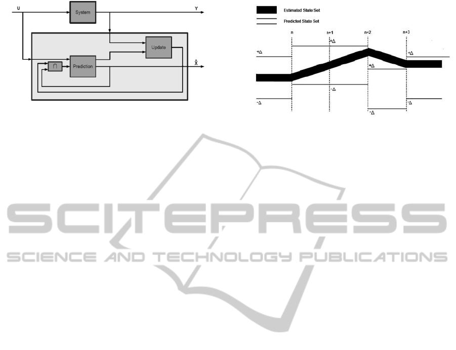
Figure 1: Diagram of the proposed observer architecture.
where
p
k
X
,
e
k
X
and
k
X
are respectively the
predicted state set, the estimated state set and the
corrected state set. The matrices A, B, C are
considered uncertain and consequently are bounded
within intervals and once again the w measurement
noise is bounded within intervals and is added to the
y measurement. Finally L is the Luenberger gain
which is defined as usual with certain systems.
The key point of this observer is the separation
of the model uncertainties and the measurement
uncertainty as in the conventional SVO; the major
difference is the Luenberger-like reconstruction of
the state from the sensor.
In order to do this, the optimal value—that is to
say the middle value—of the predicted state set is
considered in the estimation step. In this manner we
obtain, as it is the case in the SVO, a state set
considering model uncertainties and a state set
considering the sensor uncertainty. The intersection
of the two sets of data gives the correct state set.
In order to explain how this observer operates,
let us consider a model uncertainty ranging between
δ
± on all parameters of the state matrix, inducing a
±Δ enclosure on the predicted state. Figure 2 gives
a discrete-time representation of the method; this
diagram shows different cases.
At iteration n, the prediction and the estimation
are perfectly consistent and the n+1 prediction and
estimation are computed.
At iteration n+1, the prediction and the
estimation are again totally consistent; the
observation of the state is perfect. The prediction
and the estimation continue to iteration n+2.
At iteration n+2, the set of admissible
trajectories—the predicted state set—equals the n+1
predicted state set. The estimated state set should
equal the n+1 estimated state set. But, the estimated
state set deviates as it is no longer centered on the
prediction state set. This phenomenon occurs when
the parameters of the real system deviate. Indeed, as
the system is influenced by its environment, the
measurement varies and so does the state estimation.
Figure 2: Set representation of the proposed observer.
Fortunately, this case was predicted by taking
into account the uncertainties on parameters in the
prediction step. As a consequence, both the
predicted and estimated state sets are still consistent.
The next state is predicted and estimated to iteration
n+3.
At iteration n+3, the estimation deviates totally
from the prediction. The prediction and the
estimation are not consistent. This case appears
when the measurement deviates abnormally, that is
to say, out of the range admitted by the prediction—
defined according to the model uncertainties. This
simulated case corresponds to a fault. Finally, the
observation of the state continues on this manner.
To sum up, the prediction propagates model
uncertainties on the state and the estimation
computes the trajectory of the state from the sensor
measurement. If the estimation is consistent with the
prediction, the state observation continues. If the
estimation deviates beyond the frontiers predicted by
model uncertainties, a fault has appeared. This
property will be used to set up the fault detection
procedure.
As illustrated above, this observer tends to
enlarge the SVO strategy (Shamma and Tu, 1995) to
systems with missing sensors. Rather than deduce
the state directly from the sensor—supposing the
observation matrix to be invertible—the sensor is
estimated with the Luenberger approach. The
convergence of the SVLO is supported by the
correction step.
4.2 Interval Observer Convergence
Even though the correction step allows the observer
to avoid the wrapping effect, the Luenberger gain L
needs to fulfill requirements in order to ensure the
convergence of the state. As the system is uncertain,
the convergence will be studied around a box and
not around a point.
The convergence of the interval observer is
studied by considering the total error (Raïssi et al.,
ICINCO2012-9thInternationalConferenceonInformaticsinControl,AutomationandRobotics
114

2010), that is to say the error between the lower and
the upper bounds of the state:
(
)
(
)
(
)
(
)
⎡⎤
⎣⎦
We t = e t = x t - x t
(6)
If
(
)
We t
converges exponentially toward zero,
then the lower and the upper trajectories converge
toward the current state of the system. The dynamic
equation of the total error
()
We t
is described by:
(
)
(
)
(
)
(
)
(
)
(
)
(
)
()() ( ) () ()
()
We t = A - LC x t + B - LD u t + L y t + e
- A - LC x t - B - LD u t - L y t + e
(7)
Considering
(
)
ˆ
x
t
the midpoint of the set
(
)
x
t
⎡⎤
⎣⎦
:
(
)
(
)
(
)
(
)
(
)
2
⎡⎤
==+
⎣⎦
ˆ/xt mid xt xt xt
(8)
The dynamic equation (7) can be expressed as:
()
[
]
[
]
()
λ
=− +
() ()
e
We t mid A Lmid C We t t
(9)
with
()
[
]
[
]
()
[
]
et wA LwC xt wBut
λ
=− +ˆ( ) ( )
(10)
If the gain L is chosen such that
[
]
[
]
()
−mid A Lmid C
is asymptotically stable and
that
(
)
λ
et
is a positive vector
Λ
e
then the total error
converges asymptotically toward:
[] []
()
1−
=− − Λ
max
ee
WmidALmidC
(11)
Consequently, the enclosure converges toward a
box
max
e
W
. But in order to meet this requirement,
[
]
[
]
()
mid A Lmid C−
needs to be stable. Therefore,
the Luenberger gain L is determined as follows:
[] []
()
()
()
0
xy
nn
e
i
mid A Lmid C st e
L
t
abl
L
λ
≥
⎧⎫
−
⎪⎪
=∈
⎨⎬
⎪⎪
⎩⎭
\
x
(12)
4.3 Fault Detection Algorithm
The SVLO strategy has been defined and it has been
demonstrated how the state observation can be
implemented with missing sensors.
Here, we will present this observer for a fault
detection purpose. Table 1 shows the fault detection
algorithm associated with the proposed observer.
The algorithm starts by initializing the state set
k
X
to enable the beginning of the recursive
algorithm. Once the initialization has been done, a
loop is generated to compute every state set and
detect the presence of faults throughout the
simulation time.
Table 1: SVLO Algorithm.
0.
0k
X
X⇐
For
1k
=
to N
1. Compute
m
k
Y
2. Compute
p
k
X
3. Compute
e
k
X
If
pe
kk
XX
∩
≠∅
then
4.
pe
kkk
X
XX⇐∩
Else
(
)
mid
p
kk
XX⇐
End if
5. Compute
pp
kk
YCX=
If
pm
kk
YY
∩
=∅
then
6. Fault detected
End if
End for
For every loop, the following steps are repeated:
1) The measurement set is computed according to
the measurement itself and the w measurement
uncertainty. 2) The predicted state set is computed in
function of model uncertainties and the previous
corrected state set. 3) The estimated state set is
computed in function of measurement uncertainty.
4) If the intersection between the predicted state set
and the estimated state set is not empty then the set
is considered as valid. The set is assigned to the
corrected state set in order to be used at the next
iteration. Otherwise, the measurement is not
considered and is ignored. The midpoint of the
predicted state set is assigned to the corrected state
set; this prevents the algorithm from stopping when
the intersection is empty. 5) The predicted output set
is computed; it represents the image of the predicted
state set through the observation matrix. 6) If the
intersection between the predicted output set and the
measurement set is empty, a fault is detected.
Finally, the loop is finished and the next loop can be
performed.
5 NUMERICAL EXAMPLE
In order to validate the proposed method, the
following numerical example is studied.
Let us consider the linear continuous-time state
representation of a mass-spring-damper:
Reconstruction-basedSet-valuedObserver-ANewPerspectiveforFaultDetectionwithinUncertainSystems
115
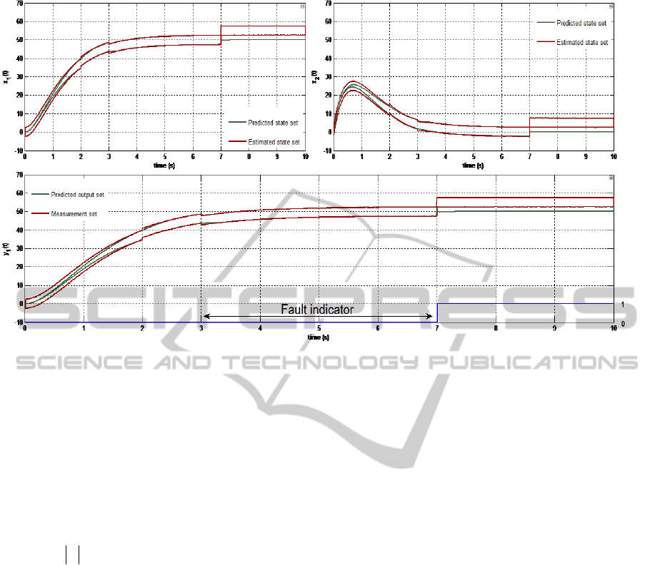
Figure 3: Observation and fault detection results for a mass-spring-damper system.
()
(
)
() () () ()
() () ()
1122
2211222
1
xt axt
x
taxtaxtut
yt x t wt
⎧
=
⎪
⎪
=++
⎨
⎪
=+
⎪
⎩
(13)
where
()()
TT
12
xx pv==x
is the state vector
representing respectively the position and the
velocity of the damper;
F=u is the input value
representing the force applied to the damper;
()
{}
5=wt|w 0.0≤w
is the ±5% measurement
noise.
12 21 22
,aaanda
are parameters of the states,
whose values are respectively
1, -2 and -3
. These
parameters are considered uncertain in what follows.
The model is discretized, the Set-Valued
Luenberger Observer is implemented and finally the
fault detection is performed.
Considering an academic example, a model
uncertainty of
±2% is added to all the state
parameters. The measurement uncertainty is
supposed to be
±5% .
In order to test the effectiveness of the proposed
fault detection method, two offsets are added to the
measurement to simulate faults. As presented in
equation (13), only the position is measured by a
sensor. Thus, the faults will be introduced on the
position measurement.
The first fault occurs between the 2-3s interval,
whereas, the second fault occurs from 7-10s. The
amplitude of the fault is around 2% of the maximum
value for the first fault and around 10% for the
second fault.
Figure 3 depicts the results obtained from the
simulations. At the top of the figure, the predicted
and estimated state sets for both the position and the
velocity states can be seen. It can be noted that the
velocity is well estimated—as intended in
Luenberger theory—even with missing sensors and
model uncertainties.
The fault detection is represented at the bottom
of Figure 3. The predicted output set and the
measurement set are computed. As previously
shown in Table I, if the intersection of both sets is
empty then a fault is detected.
If we look closely at the fault detection result, we
can report that the second fault is perfectly detected
between the 7-10s interval. But the first fault is not
detected from 2-3s. Indeed, the 2% bias fault is very
low compared to the 5% uncertainty admitted on the
sensor measurement. Therefore, the behavior of the
fault detection is totally in accordance with what
was expected. Indeed, a low bias fault is included
within the uncertainty enclosures and thus not
considered as a fault. This is why it is important at
the design stage to take into account reasonable
uncertainties to detect reasonable faults.
The SVLO gives the expected results. Its real
benefits compared to the traditional SVO are the use
of analytical redundancy to reconstruct the states.
Another interest of this approach is, this observer
does not require a matrix inversion, what allows us
ICINCO2012-9thInternationalConferenceonInformaticsinControl,AutomationandRobotics
116

to use it in a broader context than the mere SVO.
6 CONCLUSIONS
In this paper, the Set-Valued Observer has been
studied. An extension of the Set-Valued Observer
has been proposed in order to reconstruct the state
when sensors are missing. The idea is to bring
together two methods developed in different
contexts in order to make them work in synergy.
With uncertain systems, the implementation of
observer is difficult because of the wrapping effect.
This is where the Set-Valued Observer is interesting;
it can avoid this phenomenon. But the SVO is not
without drawbacks; the deduction principle of the
state implies that all measurements are available
which is not always true.
From this observation, the use of a Luenberger-
like reconstruction of the state within the SVO
seems to be a good solution. The computation of the
predicted state with model uncertainties makes it
possible to determine the set of all possible
trajectories. Then, the computation of the estimated
state with the measurement uncertainty allows the
algorithm to determine trajectories consistent with
the measurement. The intersection of the two sets
corrects the state set throughout the simulation.
Through the numerical example of the mass-
spring-damper, results have demonstrated that the
state in presence of model uncertainties can easily be
reconstructed. Moreover, the fault detection
algorithm based on the proposed observer has
demonstrated its efficacy; the observer yields the
expected results.
The Set-Valued Luenberger Observer gives
encouraging results and brings new perspectives to
the field of uncertain systems. A real-time
implementation of the observer is planned. The
Luenberger-like reconstruction of the state will
permit future work to extend fault detection to fault
isolation by implementing this observer in the form
of benches.
REFERENCES
Benothman, K., Maquin, D., Ragot, J., Benrejeb, M.,
others, 2007. Diagnosis of uncertain linear systems: an
interval approach. International Journal of Sciences
and Techniques of Automatic control & computer
engineering 1, 136–154.
Chen, J., Patton, R. J., 1999. Robust model-based fault
diagnosis for dynamic systems.
Chow, E., Willsky, A., 1984. Analytical redundancy and the
design of robust failure detection systems. Automatic
Control, IEEE Transactions on 29, 603–614.
Darengosse, C., Chevrel, P., 2002. Expérimentation d’un
observateur H∞ LPV pour la machine asynchrone.
Journal européen des systèmes automatisées 36, 641–
655.
Gertler, J., 1998. Fault Detection and Diagnosis in
Engineering Systems, 1st ed. CRC Press.
Gouzé, J., Rapaport, A., Hadj-Sadok, M., 2000. Interval
observers for uncertain biological systems. Ecological
modelling 133, 45–56.
Haimovich, H., Goodwin, G.C., Welsh, J.S., 2004. Set-
valued observers for constrained state estimation of
discrete-time systems with quantized measurements, in:
Control Conference, 2004. 5
th
Asian. pp. 1937–1945.
Henry, D., Zolghadri, A., 2005. Design and analysis of
robust residual generators for systems under feedback
control. Automatica 41, 251–264.
Jaulin, L., Kieffer, M., Didrit, O., Walter, E., 2001.
Applied Interval Analysis, 1st ed. Springer.
Kalman, R. E., 1960. A new approach to linear filtering
and prediction problems. Journal of basic Engineering
82, 35–45.
Letellier, C., Hoblos, G., Chafouk, H., 2011. Robust Fault
Detection based on Multimodel and Interval
Approach. Application to a Throttle Valve, in: IEEE
Med. Corfu, Greece
Luenberger, D. G., 1964. Observing the state of a linear
system. Military Electronics, IEEE Transactions on 8,
74–80.
Mangoubi, R. S., 1998. Robust estimation and failure
detection: A concise treatment. Springer-Verlag NY, Inc.
Ploix, S., Adrot, O., 2006. Parity relations for linear
uncertain dynamic systems. Automatica 42, 1553–1562.
Puig, V., Quevedo, J., Escobet, T., De las Heras, S., 2002.
Passive robust fault detection approaches using
interval models, in: Proceeding of the 15th IFAC
World Congress, Barcelona.
Raïssi, T., Videau, G., Zolghadri, A., 2010. Interval
observer design for consistency checks of nonlinear
continuous-time systems. Automatica 46, 518–527.
Shamma, J. S., Tu, E., 1995. Optimality of set-valued
observers for linear systems, in: Decision and Control,
1995., Proceedings of the 34th IEEE Conference On.
pp. 2081–2086.
Reconstruction-basedSet-valuedObserver-ANewPerspectiveforFaultDetectionwithinUncertainSystems
117
