PERFORMANCE ANALYSIS OF DIGITAL SLIDING MODE
CONTROLLED INVERTERS
A. Fort
1
, M. Di Marco
1
, M. Mugnaini
1
, L. Santi
1
, V. Vignoli
1
and E. Simoni
2
1
Dept of Information Engineering (DII), University of Siena, Via Roma 56, 53100, Siena, Italy
2
Borri SpA Industrial Power Solutions, Bibbiena (Arezzo), Italy
Keywords: Inverter, Sliding Mode Control, Sensitivity Analysis.
Abstract: This paper presents an analysis about the performance of bang-bang controllers used on a static machine for
energy conversion (inverter) showing their robustness with respect to some key parameters and to some
operating conditions. In particular a quasi sliding mode solution is proposed supported by sensitivity
analysis able to allow the choice of proper operative parameters set for in field testing. Moreover a
comparison between two different sliding surfaces proposal is presented.
1 INTRODUCTION
The problem of designing robust control solutions is
a well known and discussed topic present in the
literature both considering continuous (Tan, Lai and
Tse, 2012; Young, Utkin and Özgüner, 1999) as well
as discrete formulations (Gao, Wang and Homaifa,
1995; Jung, Dai and A. Keyhani, 2004; Marwali,
2004). Actually there are several papers which dealt
with the use of such controllers in the discrete time
domain applied to static conversion machines as
inverters (Jung et al., 2004; Marwali, 2004; Wong,
Leung and Tam, 1999; Gao, 1990; Hung, Gao and
Hung, 1993; Gao and Hung, 1993). Taking into
account, for example, the work of Wong et al.
(1999), such approach is limited to the application of
a solution without showing its characteristics of
robustness according to the requirements of market
regulation. Usually typical inverter static and
dynamic tests are not carried out, limiting the
possibility to argue on the effectiveness of the
control strategy on actual machine implementation.
Moreover in several works as in (Gao et al., 1995)
the behavior of the selected sliding surface is not
addressed in terms of sensitivity performance nor its
behavior for commercial employment is somehow
discussed. Starting from this points, the authors tried
to compare two control solutions based on quasi
sliding mode controllers (QSMCs) according to
some peculiar usage characteristics that are well
known in the inverter market with the final aim of
assessing some rule of thumb for the selection of the
QSMCs parameters. Actually as declared by Tan et
al. (2012) even if some works exist assessing the
performance characteristics of non linear control
systems applied to static machines, they are not
focused on the design aspects and limited to some
performance parameters. Such works of course are
useful for the industrial side because provide a path
which allow to exploit such proposal and control
strategies in real life and not only from an academic
standpoint even if some implementation aspects still
are lacking. Some others among such papers as (Tan
et al, 2012; Gao et al., 1995; Wong et al., 1999)
stress instead the accent on the importance to keep
constant, or set opportunely, the switching frequency
of the controller to improve performance or try to set
the roadmaps for correct controller switching.
Nevertheless most of these works are focused on the
design of continuous time controllers which are
likely not to be employed in everyday world. So,
starting from the work of Gao et al. (1995) and from
the one proposed by Wong et al. (1999) the authors
compared the performance of a discrete time QSMC
with an extended version proposed relying on a
higher order state description of the system of
interest which seems to better fit both the market and
designers requirements. The performance taken into
account are the ones usually considered in the
inverter market. Comments have been also carried
out considering the behaviour of a general sample
static machine in terms of sensitivity analysis with
respect to some key parameters as switching
221
Fort A., Di Marco M., Mugnaini M., Santi L., Vignoli V. and Simoni E..
PERFORMANCE ANALYSIS OF DIGITAL SLIDING MODE CONTROLLED INVERTERS.
DOI: 10.5220/0003974602210225
In Proceedings of the 1st International Conference on Smart Grids and Green IT Systems (SMARTGREENS-2012), pages 221-225
ISBN: 978-989-8565-09-9
Copyright
c
 2012 SCITEPRESS (Science and Technology Publications, Lda.)

frequency, sliding surface parameters, quasi sliding
mode band and system cutoff frequency under
nominal conditions and during static and dynamic
load variation.
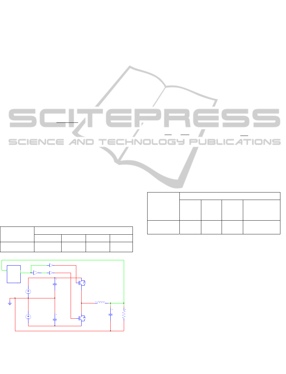
2 INVERTER STRUCTURE
In Figure 1 a typical half bridge PWM inverter
topology is sketched (Gao et al., 1995). The circuit
is composed by two constant voltage sources V
s
, a
LC group, a resistive load R
L
and a couple of IGBT
acting as power switches. The two IGBT are
controlled by a signal d(t) in counter phase, that is,
when IGBT1 is closed IGBT2 is open and viceversa
and the commanding signal determines the duty
cycle of the PWM signal defined as follows:
on off
on off
tt
d
tt
−
=
+
(1)
The switching period is set as the inverse of d/(t
on
-
t
off
). Such switching period should be smaller
compared to the circuit time constant defined by the
LC group (Gao et al., 1995). It can be easily shown
that, in such a way, the output system voltage V
out
is
a function of d and V
s
.
The parameters value for an inverter of 20kVA
are written in Table 1, where the switching
frequency of the IGBT can range typically from a
minimum value of 5kHz up to 15kHz.
Table 1: Inverter circuit parameters.
Values
L [µH] C [µF] R
L
[Ω] Vs [V]
Components
500
300 2.8 400
IGBT1
Vs
Vs
L
C RL
Cg1
Cg2
PWMVout_in
IGBT2
Vout
Figure 1: Closed control loop of an half bridge inverter
topology.
The system state space, with d as control input
and V
out
as the output, can be written in the
continuous time domain as a classical state variable
system:
yz yz
x
(t)= A x(t)+ B d(t)

(2)
where x is an n-vector and A
yz
and B
yz
are proper size
matrices for the problem to be considered and y
indicates whether the system is continuous or
discrete, while z is the state order and d is a scalar.
By choosing the state as
.
c
c
v
x=
v
⎡
⎤
⎢
⎥
⎢
⎥
⎣
⎦
(3)
where v
c
is the voltage across the capacitor, it is
possible to have a single loop feedback exploiting
the capacitor (C) voltage (v
c
) as output, assigning to
A and B the following values:
2
01
11
c
L
A=
L
CCR
⎡
⎤
⎢
⎥
⎢
⎥
⎢
⎥
−−
⎢
⎥
⎣
⎦
;
2
0
c
c
B=
V
LC
⎡⎤
⎢⎥
⎢⎥
⎢⎥
⎢⎥
⎣⎦
(4)
Figures of merit of a commercial system as the
one described should be within the limits of Table 2
in order to have a competitive features in the energy
market.
Table 2: Commercial performance benchmark parameters.
Parameters
for 20kVA
Values
THD
(*)
Power
Factor
Static
load
change
dynamic (0-
100%) load
change
<2% 0.99 ±1%
±5% <10 ms
recovery time
(*)
These figures are in accordance with IEC6204-1-3 and are
expressed for linear load in voltage instead of current
3 CONTROL THEORY AND
DESIGN OF THE SWITCHING
FUNCTION
3.1 Control Basics
The main concept of sliding mode control exploits
the definition of a sliding surface and a proper set of
parameters that enable such surface to become
globally attractive for the system under
consideration. Given the state–space representation
(4), in order to derive a sliding mode control the
sliding manifold:
0S(x(t))=
(5)
SMARTGREENS2012-1stInternationalConferenceonSmartGridsandGreenITSystems
222

should satisfy the following inequality
.
0S(x(t))
<
(6)
while a suitable control law of the form:
d =
0
0
+
d S(x(t))>
d S(x(t))<
−
⎧
⎨
⎩
(7)
should guarantee each state trajectory to converge to
(5) (Tan et al., 2012;Young et al., 1999; Gao et al.,
1995; Jung et al., 2004; Marwali, 2004; Wong et al.,
1999; Gao, 1990; Hung et al., 1993; Gao and Hung,
1993).
In other words, equations (5) to (7) and the right
choice of d assure that the state vector, starting from
any initial condition, will slide up to the null
solution.
A common choice for the reaching law, is given
by Gao et al. (1995):
sgnS(x(t))= qS(x(t)) ε (S(x(t)))−−

(8)
where q and ε are positive quantities opportunely
chosen in order to guarantee the system global
stability.
3.2 Digital Control for Static Machines
The problem described in the previous section can
be applied with suitable manipulations and
assumptions to the discrete time case (DTC).
Considering the discrete form of the system
represented in (2), sampled at instant T
k
(represented
from now on as x(T
k
)= x(k)) it is possible to write
(4) as:
1
dz dz
x
(k + )= A x(k)+ B d(k) (9)
where A
dz
and B
dz
are the discrete forms according to
classical system theory as argued by D’Azzo and
Houpis (1995):
0
and
T
k
AA
cz k cz k
dz dz
TT
A=e ; B= e Bdτ
∫
(10)
Together with the discrete time representation of
the system the entire domain must be discrete. Some
authors, among whom the first has been Hoft,
suggested a discrete representation of the continuous
time convergence law described by the following:
[
]
1
0
k+ k k
S(x ) S(x ) S(x ) <−
(11)
Other formulations, which result in a better
implementation of the previous concept for discrete
time controllers (DTC), are presented in the
literature (see, e.g., Gao et al. (1995) and references
therein). A possible choice for the discrete-time
form of (8) is:
1sgn
ss
S(k + ) S(k)= qT S(k) εT(S(k))=(k)
φ
−− −
(12)
where T
s
is the switching period and the quantity qT
s
must satisfy qT
s
<1 in order to guarantee that,
starting from any initial condition, the trajectories
will move to the sliding surface.
3.3 System Switching Law
Once the reaching law is defined as per (12), a
switching function should be chosen in order to let
(7) in its discrete formulation to be a valid statement.
By selecting S(k) as a linear combination of the
state variables:
10
T
w
S(k + )= S(k)= = Φ x(k)
, (13)
where Φ
w
is a vector of scalars of dimension (w) it is
possible to write (8) as:
sgn
TT
sw s w
(k)= qT Φ x(k) εT(Φ x(k)) φ −−
(14)
and consequently (13) as:
11
TT
ww
TTT
www
S(k + ) S(k)= Φ x(k + ) Φ x(k) =
Φ Ax(k)+Φ Bd(k) Φ x(k) = (k)
φ
−−
=−
(15)
which, in turns, provides an expression for the
switching law d(k):
(
)
(
)
1
TT T
ww w
d(k)= Φ B Φ Ax(k) Φ x(k) (k) φ
−
−−−
(16)
By replacing in (13) the state x(k) with the error
e(k) among the state itself and a reference signal, it is
possible to design a suitable sliding manifold for the
systems as the one of Figure 1. Note that when the
system moves on a sliding surface it behaves as a
linear system approaching the null solution with time
constants depending on the choice of the vector Φ
w.
4 DIGITAL CIRCUIT CONTROL
Aim of this section is the design of the control law
and the sliding manifold for the circuit described in
Section I, according to (13). Using the output
voltage error (with respect to a reference signal x
r
(t))
, it can be easily verified that the
evolution of e
2
(t) i.e.
.
2
()
()
()
et
et=
et
⎡
⎤
⎢
⎥
⎢
⎥
⎣
⎦
(17)
[
] x(t)(t)x=e(t)
r
−
PERFORMANCEANALYSISOFDIGITALSLIDINGMODECONTROLLEDINVERTERS
223

obeys to (2) and (4). It is therefore possible to extend
the state representation of (2) by defining matrices
A
c3
and B
c3
as follows:
⎥
⎥
⎥
⎥
⎥
⎥
⎦
⎤
⎢
⎢
⎢
⎢
⎢
⎢
⎣
⎡
=
⎥
⎥
⎥
⎥
⎥
⎥
⎥
⎦
⎤
⎢
⎢
⎢
⎢
⎢
⎢
⎢
⎣
⎡
−−
=
⎥
⎥
⎥
⎥
⎥
⎥
⎥
⎥
⎥
⎥
⎥
⎥
⎦
⎤
⎢
⎢
⎢
⎢
⎢
⎢
⎢
⎢
⎢
⎢
⎢
⎢
⎣
⎡
=
∫
LC
V
B
CRLC
A
te
te
)dτe(τ
te
s
c
L
c
t
0
0
;
11
0
100
010
;
)(
)(
)
)(
33
.
0
3

(18)
Since (2) and (18) admit their discrete-time
counterpart, once they are replaced in (16), it is
possible to design the control signal d(k).
5 CIRCUIT PERFORMANCE:
SENSITIVITY ANALYSIS
The circuit in Figure 1 has been simulated using
PSIM 9.0.4 software and the system characteristics
in terms of commercial performance of the two
parameter sliding manifold have been analyzed. The
nominal system parameters for simulations are:
switching frequency of f
s
=10kHz; sampling
frequency f
k
=1MHz, qT
s
=0.25; εT
s
=0.1; sliding
surface parameters for the 2D approach Φ
2
=( Φ
1
=1,
Φ
2
=10
-6
); sliding surface parameters for the 3D
approach Φ
3
=( Φ
1
=1, Φ
2
=1, Φ
3
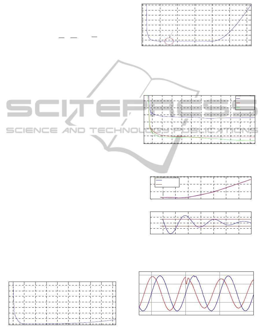
=0,0625). In Figure 2,
3 and 4 the system performance in terms of voltage
THD% with respect to two dimensional manifold
slope variation, system cutoff frequency (C only)
variation and switching frequency variation have
been reported, respectively. In Figure 5 it is shown
how the system performance, during dynamic load
variation (from 0-100% of the nominal load), can be
slightly improved in terms of settling time changing
the ε parameter which is justified by the change into
the QSMC band. According to Figure 6 the static
behaviour of the two parameters controller is
generally worse with respect to the choice of the
three parameters sliding surface while the two
sliding controllers have almost the same dynamical
0 1 2 3 4 5 6 7 8 9
x 10
-6
1.5
1.6
1.7
1.8
1.9
2
2.1
2.2
THD vs.
φ
2
;
φ
1
= 1
THD [%]
φ
2
Figure 2: THD% variation with respect to the change in
the slope of the QSMC in the 2D error state space.
behaviour which is generally better with respect to
traditional PID systems (Gao et al., 1995).
0 200 400 600 800 1000 1200
1.4
1.6
1.8
2
2.2
2.4
2.6
2.8
3
THD vs. C
THD [%]
C [uF]
THD
min
(C=300 uF)
Figure 3: THD% variation with respect to the change into
the system cutoff frequency. This is important from a
design standpoint showing the possibility to reduce the
weight and space occupation of such capacitor keeping the
same performance.
100 150 200 250 300 350 400 450 500 550 600
0.8
1
1.2
1.4
1.6
1.8
2
THD vs. C
THD [%]
C [uF]
f
s
= 5 kHz
f
s
= 10 kHz
f
s
= 15 kHz
Figure 4: THD % variation with respect to C and
evaluated a three switching frequencies.
0.049 0.05 0.051 0.052 0.053 0.054 0.055 0.056 0.057
-400
-200
0
200
ε
T
s
= 10 (
ε
T
s
=0.1 d esign)
V
out
[V]
Time [s]
V
out
(ALV)
V
out
0.049 0.05 0.051 0.052 0.053 0.054 0.055 0.056 0.057
-20
-10
0
10
20
Settling time within 2%
|V
out
- V
out
(ALV) | [V]
Time [s]
Figure 5: System dynamic response to load variation (0-
100% Vout-Vout AVL after load variation) with ε
parameter 100 times greater than the design one .
0.04 0.06 0.08
Time (s)
Vout_2_param manifold Vout_3_param_manifold
Figure 6: Comparison between systems performance (static
behavior 0-100% load) with two parameters (red) and three
parameters (blue) controllers. The phase shift has been
magnified to make two picture easily comparable.
SMARTGREENS2012-1stInternationalConferenceonSmartGridsandGreenITSystems
224

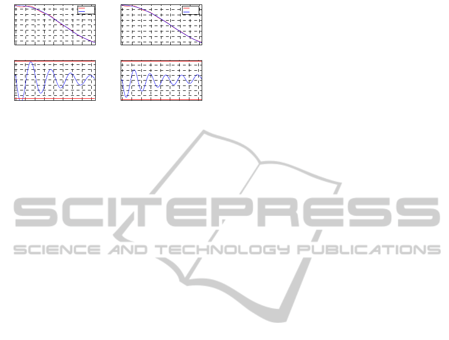
0.065 0. 066 0.067 0.068 0.069 0.07 0.071 0.072 0.073
-300
-200
-100
0
100
200
300
Two Parameters Sl iding Manifold
V
out
[V]
Tim e [ s ]
V
out
ALV
V
out
0.065 0.066 0.067 0.068 0. 069 0.07 0.071 0.072 0.073
-15
-10
-5
0
5
10
15
Settling Time Within 2%
|V-V
r
| [V]
Tim e [ s]
0.065 0.066 0.067 0.068 0.069 0. 07 0. 071 0.072 0.073
-300
-200
-100
0
100
200
300
Three Parameters Sl iding Manifold
V
out
[V]
Time [s]
V
out
ALV
V
out
0.065 0. 066 0.067 0.068 0.069 0.07 0.071 0.072 0.073
-15
-10
-5
0
5
10
15
Sett ling Time W ithin 2%
|V-V
r
| [V]
Ti [ ]
Figure 7: Dynamic behavior of the two parameter
controller (left) with respect to the three parameters one
(right).
6 CONCLUSIONS
In this work the authors, starting from an existing
circuit model, have simulated the performance of
two sliding manifolds applied to a commercial
designed inverter of 20kVA. The authors identified
that there are differences between control
implementations that are evident upon static load
variation and are less evident under dynamic ones.
Simulations have been carried out in order to
minimize the chattering due to finite switching
frequency (coping with actual implementation on
IGBTs) and taking into account the possibility to act
on the ε parameter to control the admissible band.
REFERENCES
S. C. Tan, Y. M. Lai and C. K. Tse, 2012. Sliding Mode
Control of Switching Power Converters. CRC Press.
K. D. Young, V. I. Utkin and Ü. Özgüner, 1999. A
Control Engineer’s Guide to Sliding Mode Control.
IEEE Transactions on Control Systems Technology, 7,
328-342.
W. Gao, Y. Wang and A. Homaifa, 1995. Discrete-Time
Variable Structure Control Systems. IEEE
Transactions on Industrial Electronics, 42, 117-122.
J. W. Jung, M. Dai and A. Keyhani, 2004. Optimal
Control of Three-Phase PWM Inverter for UPS
Systems. 35th Annual IEEE Power Electronics
Specialists Conference, 2054-2059.
M. N. R. Marwali, 2004. Digital Control Of Pulse Width
Modulated Inverters For High Performance
Uninterruptible Power Supplies. PhD Thesis, Ohio
State University.
L. K. Wong, F. H. F. Leung and P. K. S. Tam, 1999.
Control of PWM Inverter using a Discrete-time
Sliding Mode Controller. IEEE International
Conference on Power Electronics and Drive Systems,
PEDS’99, 947-950.
W. B. Gao, 1990. Foundation of Variable Structure
Control. Beijing: China Press of Science and
Technology.
J. Y. Hung, W. B. Gao and J. C. Hung, 1993. Variable
Structure Control: A survey. IEEE Transactions on
Industrial Electronics, 40, 2-22.
W. B. Gao and J. C. Hung, 1993. Variable Structure
Control of Nonlinear Systems: A new approach. IEEE
Transactions on Industrial Electronics, 40. 45-55.
J. J. D’Azzo and C. D. Houpis, 1995. Linear Control
System Analysis and Design. McGraw-Hill Higher
Education.
PERFORMANCEANALYSISOFDIGITALSLIDINGMODECONTROLLEDINVERTERS
225