Flow Optimization for Iron Ore Reclaiming Process
Bruno Eduardo Lopes, José Pinheiro de Moura, Denis Anderson Ribeiro,
Fernando Henrique Costa e Borges and Marco Antônio de Souza
VALE, Av. dos Portugueses, 1000 Boqueirão, CEP 65085-580, São Luis, MA, Brazil
Keywords: Iron Ore Reclaimers, PID Control, Process Flow, Predictive Control.
Abstract: The purpose of the this paper is to demonstrate the optimization of the flow for the iron ore reclaiming
process by reclaimers over rails using implementation of PID control algorithms, identification techniques,
Predictive Control and a new effort-based learning method herein called reinforcement by difference
learning method and proportional reinforcement learning method. The outcome was an increase of
productivity, with reduction of the flow variability and on the amount of overflow occurrences.
1 INTRODUCTION
The need to control physical processes and systems
exist since remote times. The manual control, first
way for controlling used by man and still found in
many processes nowadays, shows the need of a
human operator that must know the system and have
reasonable experience and skills. With the
sophistication increase of human activities came
along the interest and necessity to automate or semi-
automate some processes, this was possible due to
the scientific and technological development that
among some several other knowledge brought us the
classical control theories. However, with the
advance of technology, systems and processes
became more complex making ineffective, or even
impossible, the usage of conventional controllers
obtained from classical theories. This initiated a
search for new methods and strategies for control
such as: multivariable control, adaptive control,
predictive control and intelligent systems control.
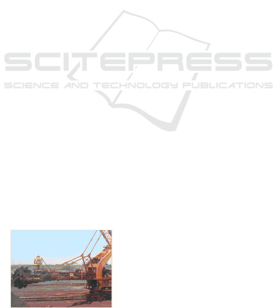
Figure 1: Stacker-Reclaimer at TMPM.
This paper demonstrates the application of
techniques for identification and process control n
stacker-reclaimers/reclaimers over rails located at
Terminal Maritimo Ponta da Madeira (TMPM).
The Terminal Maritimo Ponta da Madeira,
located in Brazil at the city of São Luis-MA, belongs
to VALE and is composed, currently, by 4 car
dumpers with nominal capacity of 8,000 tons per
hour, ten iron ore stock yards, conveyor belts and 10
yard machines divided in: 3 stackers, 3 reclaimers, 4
stacker/reclaimer and 4 ship loaders, all used to ship
iron ore.
2 OPERATIONAL MODES FOR
RECLAIMING
Reclaimers installed at TMPM can use 3 (three)
modes to control the reclaiming process:
Local
Manual
Semi-Automatic
The work for optimization was done to improve
the performance only for the semi-automatic
operation mode.
2.1 Local Mode
This mode purpose is for maintenance or testing and
will be executed through action from the
maintenance technicians on the command buttons
located nearby the equipments and respecting all the
security interlocks, not being possible in this mode
425
Eduardo Lopes B., Pinheiro de Moura J., Anderson Ribeiro D., Henrique Costa e Borges F. and Antônio de Souza M..
Flow Optimization for Iron Ore Reclaiming Process.
DOI: 10.5220/0003975404250432
In Proceedings of the 9th International Conference on Informatics in Control, Automation and Robotics (ICINCO-2012), pages 425-432
ISBN: 978-989-8565-21-1
Copyright
c
2012 SCITEPRESS (Science and Technology Publications, Lda.)

any productive process. All equipments are
commanded via the CLP.
2.2 Manual Mode
In order to characterize the manual mode, only is
needed to have selected on the HMI or in the SOS
(system operating station), the operation from
CABIN or CONTROL ROOM and, additionally,
have been selected the MANUAL mode. The
signaling will be through MANUAL OPERATING
ROOM or MANUAL CABIN written on the
operating screen.
The reclaiming will be under the command of
the operator through the usage of the levers at the
console. In this mode also the security and process
interlocks are respected, disallowing start them out
of sequence.
The translation movement will not revert
automatically and, the material reclaiming can be
done in any area of the stock yar d as long as the
operator detects it available.
The equipments will be commanded individually
via CLP, as long as the yard’s conveyor belt is on
(Start Conveyor of Spear and Start Bucket Wheel)
2.3 Semi-Automatic Mode
In this operating mode, the operator establish the
parameters of the process such as initial and final
landmark, set point for the reclaiming flow rate and
the time or distance for advancing and the angles for
the reversal of spear rotation.
Initially, through the rotation lever, the
movement is commanded and reversal points are
marked. The marked points are memorized and after
this marking, every time the rotation angle reaches
these points, there is a reversion of this movement.
Through the operating console it is possible to reset
the information of reversal points previously
defined, allowing a new preset for adjustment of the
reversal point.
In this mode, the backing movement and spear
descent for changing the reclaiming stand are done
manually, being necessary reinitiate de reclaiming
process, marking new reversal points for the spear
rotation.
The rotation speed is controlled through a PID
control loop and the time for the translation step is
determined by the operator as well as may be
adjusted automatically by a logic developed on the
CLP.
In order to preserve the flow measurement
without the interference of the material’s impact that
is being reclaimed to the spear conveyor belt, the
scale is mounted a reasonable distance from the
bucket wheel, generally in the middle of the spear’s
conveyor belt. This distance of the scale to the
bucket wheel causes an average delay of 10 seconds
and for this reason the flow measured by the scale is
not used as process variable.
3 STANDARD LOGIC FOR FLOW
OPTIMIZATION
The standard logic for flow optimization existing on
TMPM was developed aiming the control of the
following variables:
Rotation speed
Translation step
3.1 Rotation Speed Control
3.1.1 Mathematic Data Modeling
Due to the high elevated delay of the bucket wheel
in relation to the process scale according to figure 2,
which prevents the deployment of a flow control, it
was necessary develop a mathematic model to
estimate the reclaiming flow and eliminate this
delay, known as Dead Time (Smith, 1957; Astrom et
al., 1994; Hagglund, 1992).
Initially was analyzed the correlation of the flow
with the following process variables:
Current or pressure of the bucket wheel.
Current of the rotation engine.
Rotation speed
It was noted the existence of a high correlation
between the reclaiming flow and the current or
pressure of the bucket wheel and low correlation in
regards to the current and speed of the rotation. So,
only the current or pressure of the bucket wheel was
used for estimating the reclaiming flow.
In order to represent mathematically the
estimated reclaiming flow it was used the ARX
linear model which concepts are well demonstrated
in Aguirre (2007) and the extended minimum square
method (Aguirre, 2000) to estimate the parameters.
In order to determine the order of the model the auto
values analysis model, created by Lopes et al.
(2010), was utilized.
ICINCO 2012 - 9th International Conference on Informatics in Control, Automation and Robotics
426
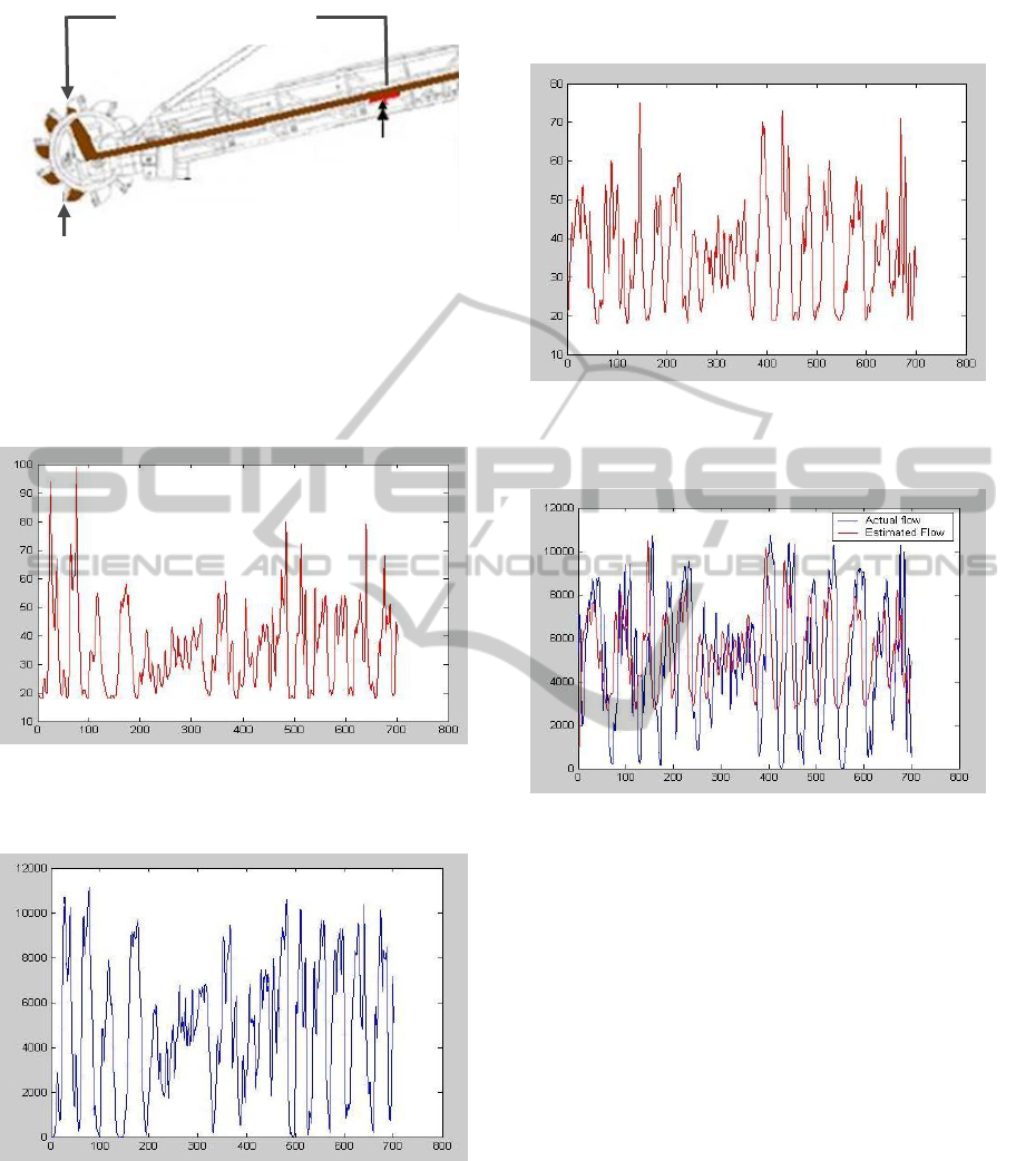
Figure 2: Delay between bucket wheel and the scale.
In order to estimate the parameters of the ARX
model used data from current (input) and flow
(output) as shown in figures 3 (current of the bucket
wheel) and 4 (flow).
Figure 3: Data of current of the bucket wheel for
estimating the model parameters (Axis x=number de
samples / Axis y= current of the bucket wheel in Amper).
Figure 4: Data of flow for estimating the model
parameters (Axis x=number de samples / Axis y= flow in
Ton/h).
The 3° order model obtained was:
y(k) = 0,09y(k-3) - 0,76y(k-2) + 1,546y(k-1)
+ 12,11u(k-2) – 36,48u(k-1) + 43,238u(k)
(1)
For the model 1 validation it was used the data
from the current of the bucket wheel and flow shown
on the figures below.
Figure 5: Data of current of the bucket wheel for
validation of model 1 (Axis x=number de samples / Axis
y= current of the bucket wheel in Amper).
Figure 6: Comparison of actual flow with estimated (Axis
x=number de samples / Axis y= flow in Ton/h).
The obtained flow and the estimated flow for
current’s data as seen on figure 5 are shown on
figure 6. It can be noted that the estimated has a
good representation of actual data.
3.1.2 Reinforcement Learning
Due to a change on the behavior of the current of the
reclaimer’s bucket wheel over time, the model 1 did
not estimate the flow correctly any longer. The
problem is verified a month after the system was
modeled.
To fix this problem a new learning by
reinforcement method was created called
reinforcement by difference learning method and
proportional reinforcement learning method. The
procedure for utilizing this method is:
a. Analyze graphically the behavior of the real
data with the data estimated by the
mathematical model. Divide the graph in two
Scale
Bucket Wheel
TIME = +/- 10 Seconds
Flow Optimization for Iron Ore Reclaiming Process
427
or more areas, and these areas may be
divided in accordance with a possible change
in the behavior observed between actual and
estimated data. On this work, it was divided
in 3 areas: Area 1: Flow < 4000 t/h; Area 2:
Flow >= 4000 t/h e <=8000 t/h; Area 3:
Flow>8000 t/h.
b. Should the difference found between the
actual and estimated data are just a stationary
error choose the reinforcement by difference
learning method. Should it is an error of
proportionality use the proportional
reinforcement learning method. On this work
the reinforcement by difference learning
method was used.
c. Should the reinforcement by difference
learning method is opted, compare the
delayed estimated data (according to the
delay) with actual data, determine the
difference between them (Actual data –
Estimated data) and sum this difference to
the estimated data. This difference should be
calculated separately for each area
determined on item a.
d. Should proportional reinforcement learning
method is opted compare the delayed
estimated data (according to the delay) with
actual data, divide them (actual data /
estimated data) and multiply the obtained
value to the estimated value. This division
should the calculated separately for each area
determined on item a.
e. The calculation error between actual data and
estimated data should be done every n
seconds, being that the value of n will be
determined according to the problem to
solved. On this work it was used n=10
seconds.
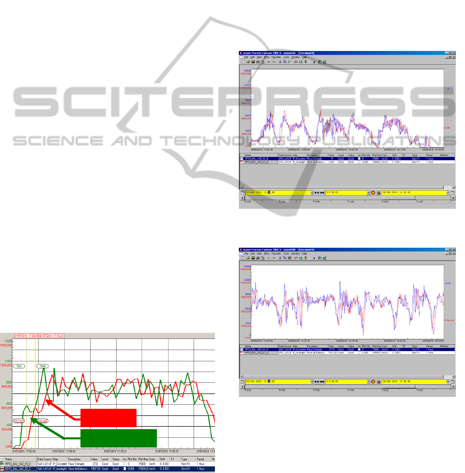
Figure 7: Estimated flow and actual flow comparison
(Axis x=Time / Axis y= flow in Ton/h).
The model 1 and the reinforcement learning
method was configured on the CLP of the reclaimer
and at figure 7, data extracted from the PIMS, can be
verified that the estimated flow has a good
representation of the actual flow.
By the usage of the reinforcement by difference
learning method on reclaimers and stackers-
reclaimers of TMPM was possible to ensure
accuracy of the estimated flow no matter the
difference of the behavior of the bucket wheel over
time. This accuracy can be verified on figure 8, 9
and 10 that during several months presented an
estimated flow (blue) very close the actual flow
(red) keeping the delay time.
Figure 8: Comparison of actual flow and estimated flow
on 08/20/2010 (Axis x = time / Axis y= flow in Ton/h).
Figure 9: Comparison of actual flow and estimated flow
on 09/20/2010 (Axis x = time / Axis y= flow in Ton/h).
Actual flow
Estimated flow
Delay = 12s
ICINCO 2012 - 9th International Conference on Informatics in Control, Automation and Robotics
428
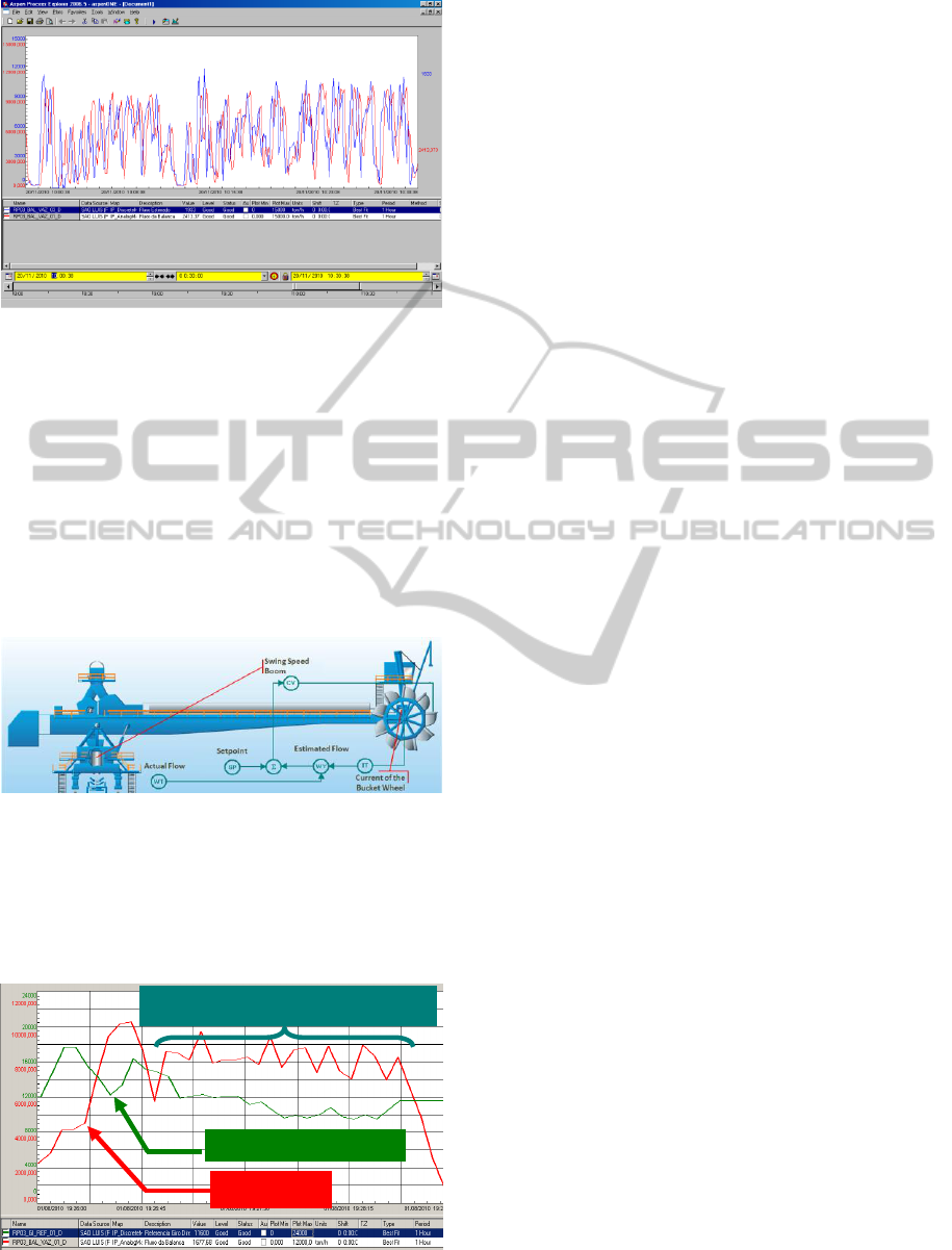
Figure 10: Comparison of actual flow and estimated flow
on 11/20/2010 (Axis x = time / Axis y= flow in Ton/h).
3.1.3 PID Control
The rotation speed - which interferes on the intensity
of the penetration of the bucket wheel in the pile – is
defined through a PID control loop that has as set
point (SP) the rate of the desired reclaiming flow
and as process variable (PV) the estimated flow
through the current of the bucket wheel’s engine.
The controlled variable (CV) is the Swing Speed
Boom. The control loop can be verified on figure 11.
Figure 11: Control loop of the flow.
As the method for tuning the PID was not the
purpose of this paper, it was used a practical tuning
method and the parameters found were kp Gain =
0.3; ki Gain = 0.2; Sample Period = 100
milliseconds.
Figure 12: Flow controlled at 8000 ton/h (Axis x = time /
Axis y= flow in Ton/h).
The PID control and the parameters found were
deployed on CLP of the reclaimer and the result is
demonstrated on figure 12 in which the operator has
established as set point value of 8000 t/h and the
PID controller adjusted the rotation speed until the
desired flow has been reached. For this PID was
setup a dead band of 500 t/h.
3.2 Translation Step
The initial translation step is manually defined by
the operator and individually each direction for the
rotation movement (clockwise and counter clock
wise). Its adjustment is made according to time or
distance for the translation in seconds or
centimeters.
If the operator chooses the automatic control of
the translation step, the ideal step is calculated
according of the average rotation speed that the
reclaimer needed to reach the setpoint value of the
flow during one of the rotation direction. If the
average speed of the rotation to achieve the desired
flow is elevated the time or distance of the
translation step is increase, if it is too low the time or
distance of the translation step is reduced.
The higher the translation step the lower will be
the rotation speed necessary for the reclaimer to
reach the set point and smaller will the loses caused
by the inversion of the rotation direction. On the
other hand, higher will be the possibility of overflow
occurrences and overloads on the bucket wheel. The
lower the translation step the higher will be the
rotation speed necessary for the reclaimer to achieve
the set point causing more loses due to the inversion
of the rotation direction. The idea is to adjust the
translation step in order to make the desired flow to
be achieved at a determined ideal speed in each
rotation.
The logic for translation step control was
configured on the CLP’s reclaimer and the result is
verified on figures 13 and 14. Before the
implementation of translation step control the
rotation in each direction, at base layer, has taken
about 2 minutes, as shown on figure 13. After the
implementation of the translation step control, the
rotation in each direction, at base layer, turned out to
take an average of 5 minutes, figure 14, reducing
loses due to changes on the direction of the rotation
and increasing productivity.
Flow controlled at 8000 ton/h
Controlled flow
Rotation speed reduction
Flow Optimization for Iron Ore Reclaiming Process
429
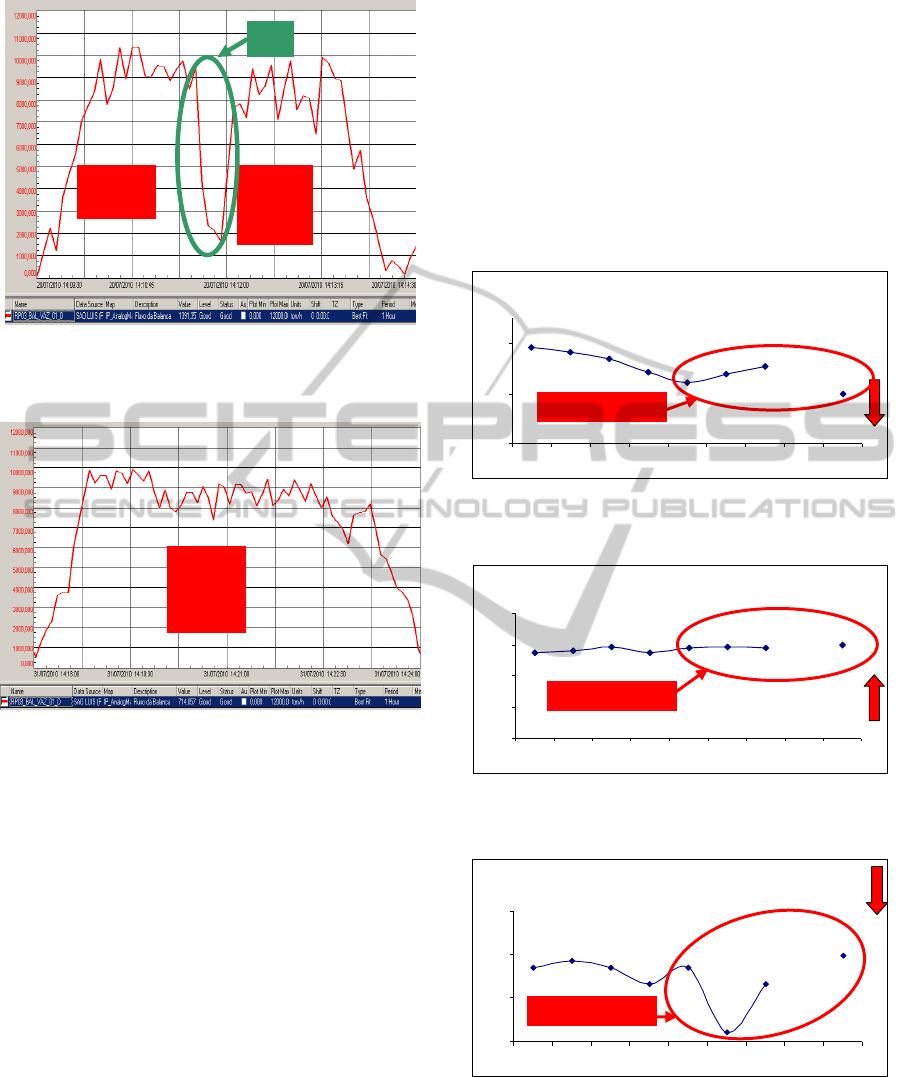
Figure 13: Time in each direction before implementation
of the translation step control (Axis x = time / Axis y=
flow in Ton/h).
Figure 14: Time in each direction after implementation of
the translation step control (Axis x = time / Axis y= flow
in Ton/h).
4 OUTCOMES
The purpose of this paper for optimization of
reclaimer flow control is the increase of productivity
along with decrease of variability and overflow
rates.
The variability or coefficient of variation (Cv) is
calculated dividing the standard deviation (σ) by the
flow average (µ):
Cv = σ / µ
(1)
At TMPM, overflow is considered as a
reclaiming flow over 10,000t/h during a period
higher or equals to 5 seconds.
In this paper will be demonstrated the results
obtained with the deployment of the optimization
work of flow control of the reclaimer RP-313K-03
and the Stacker-reclaimer ER-313K-04. The same
work was developed for the other yard machines of
TMPM and similar results were found.
4.1 RP-313K-03
On figures 15, 16 and 17 it is possible to notice that
after the implementation of the flow control
optimization for RP-313K-03 was obtained an
average increase of 5% in productivity along with
average reduction of 10% in variability and 20% on
overflow occurrences.
Varibialidade - RP 313 - 03
0,35
0,44
0,43
0,42
0,39
0,39
0,37
0,40
0,25
0,35
0,45
mai/10 jun/10 jul/10 ago/10 set/10 out/10 nov/10 dez/10 jan/11
Figure 15: Variability evolution of RP-313K-03 (Axis x =
time / Axis y= variability).
Fluxo - RP 313 - 03
5791
5778
5867
5501
5846
5588
5452
5981
0
2000
4000
6000
8000
mai/10 jun/10 jul/10 ago/10 set/10 out/10 nov/10 dez/10 jan/11
Figure 16: Flow evolution of RP-313K-03 (Axis x = time /
Axis y= flow in Ton/h).
Sobrefluxo - RP 313-03
5,3
7,9
6,8
7,4
6,8
0,9
6,8
5,3
0,0
4,0
8,0
12,0
mai/10 jun/10 jul/10 ago/10 set/10 out/10 nov/10 dez/10 jan/11
Figure 17: Overflow evolution of RP-313K-03 (Axis x =
time / Axis y= overflow occurrences).
4.2 ER-313K-04
For the ER-313K-04 the result was even better, thus,
as demonstrated on figures 18, 19 and 20 there was
Clockwise
rotation
Counter
clockwise
rotation
Counter
Clockwise
rotation
Loses
New pattern
New pattern
New pattern
ICINCO 2012 - 9th International Conference on Informatics in Control, Automation and Robotics
430
an average increase of 9% in productivity along with
average reduction of 20% on variability and 39% on
overflow occurrences.
Varibialidade - ER 313 - 04
0,31
0,30
0,43
0,39
0,38
0,34
0,41
0,38
0,32
0,25
0,35
0,45
mai/10 jun/10 jul/10 ago/10 set/10 out/10 nov/10 dez/10 jan/11
Figure 18: Variability evolution of ER-313K-04 (Axis x =
time / Axis y= variability).
Fluxo - ER 313 - 04
6343
6149
5546
5997
5589
5630
5842
5412
6153
0
2000
4000
6000
8000
mai/10 jun/10 jul/10 ago/10 set/10 out/10 nov/10 dez/10 jan/11
Figure 19: Flow evolution of ER-313K-04 (Axis x = time /
Axis y= flow in Ton/h).
Sobrefluxo - ER 313-04
13,5
7,0
7,5
14,0
7,3
9,2
16,1
15,6
3,2
0,0
4,0
8,0
12,0
16,0
20,0
mai/10 jun/10 jul/10 ago/10 set/10 out/10 nov/10 dez/10 jan/11
Figure 20: Overflow evolution of ER-313K-04 (Axis x =
time / Axis y= overflow occurrences).
5 PREDICTIVE CONTROL
In order to improve the flow control in 2011 was
developed a solution that is based on predictive
control techniques (Camacho and Bordons, 1999).
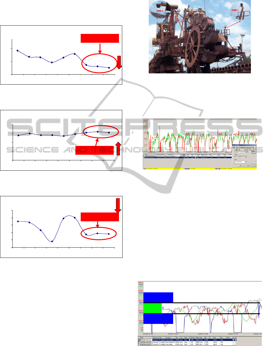
To develop the predictive control, radar-like
sensors were installed alongside the bucket wheel, as
shown on figure 21.
Those sensors tell to the system the penetration
distance of the bucket wheel into the pile and the
height that is been reclaimed. By using this
Figure 21: Radar-like sensors installation localization.
information along with the spin speed data it was
possible to develop an estimator to predict the flow
to be reclaimed. The comparison of the expected
flow versus the actual one is shown on figure 22.
Figure 22: Comparison of actual flow (Green) and
expected flow (Red) on 02/12/2011 (Axis x = time / Axis
y= flow in Ton/h).
After the sensors were installed a logic was
developed to verify the expected flow values and
should it be higher or lower 15% of a desired flow a
predictive control action is triggered, in other words,
the PID flow controller is deactivated temporarily,
the ideal speed reference calculated by the predictive
control is written on the PLC and then the PID
controller is reactivated. It is important to mention
that the PID controls the flow that was estimated
using the current or pressure of the bucket wheel as
inputs. The action area covered by the controller is
demonstrated on figure 23.
Figure 23: PID and Predictive control action area.
Predicted flow (Blue). Estimated flow (Green) and Actual
flow (Red). (Axis x = time / Axis y= flow in Ton/h).
Predictive
Predictive
PID
New pattern
New pattern
New pattern
Flow Optimization for Iron Ore Reclaiming Process
431

The productivity gains with the implementation
of the predictive control can be seen on figure 24
where area 1 represents the productivity values for
the manual operation, area 2 represents the
productivity values using only the PID control and
area 3 represents the productivity obtained by using
the predictive control. The improvements obtained
are 11% over the manual operation and 6% over the
isolated usage of the PID control.
PRODUTIVIDADE
5787
6043
5825
6759
6691
6300
6458
6120
5707
6050
6339
5712
5875
6120
5812
6233
5645
6036
6187
5491
5804
5963
5889
5793
5612
5883
5928
6133
5916
6048
6334
6140
6330
6090
5315
5000
5500
6000
6500
7000
4-nov
6-nov
8-nov
11-nov
14-nov
21-nov
24-nov
26-nov
28-nov
30-nov
2-dez
4-dez
8-dez
12-dez
16-dez
19-dez
21-dez
23-dez
25-dez
5884
6157
6530
1
2
3
Figure 24: Productivity improvements with the utilization
of the predictive controller. (Axis x = time / Axis y= flow
in Ton/h).
6 CONCLUSIONS
The outcomes shown in this paper demonstrated that
the new pattern adopted by Vale for the iron ore
reclaiming process at TMPM, brought a significant
increase of productivity for its operations.
Additionally to the gain in productivity, it was
possible to obtain a reduction in operational loses on
the reclaiming process with reduction of overflow
occurrence.
Due to the obtained gains, this new pattern for
flow control developed at TMPM was established as
a standard to be used by the other Vale’s ports.
REFERENCES
Aguirre, L. A., 2000. A nonlinear dynamical approach to
system identification, IEEE Circuits & Systems
Society Newsletter 11(2): 10-23, 47.
Aguirre, L. A., 2007. Introdução a Identificação de
Sistemas. Técnicas Lineares e Não Lineares Aplicadas
a Sistemas Reais. Editora UFMG, Belo Horizonte -
MG. Brasil, 3a edição.
Lopes, B. E, Corrêa, M. V., Teixeira, R. A. and Moura, J.
P., 2010. Método de Análise dos Autovalores para
seleção de ordem de modelos lineares. Anais do 18º
Congresso Brasileiro de Automática, Bonito MS, pp.
498—504
Astrom, K., Hang C., Lim, B., 1994. A New Smith
Predictor for Controlling a Process with a Integrator
and Long Dead Time. IEEE Transaction on Automatic
Control 39(2): 343-345
Hagglund, T., 1992. A Predictive PI Controller for
Processis with Long Dead Time. IEEE, Control
Systems, pp57-60.
Smith, O. J. M., 1957. Closed Control of Loops With
Dead-Time, Chem. Eng. Progress; 53:217-219.
Astrim, K. J., Hagglund T., PID Controllers: Theory,
Design, and Tunning. 2ª Edition, Instrument Society of
America, 1995.
Camacho, E., Bordons, C., 1999. Model Predictive
Control. Springer Verlag.
ICINCO 2012 - 9th International Conference on Informatics in Control, Automation and Robotics
432
