
On the Multiple-view Triangulation Problem with Perspective and
Non-perspective Cameras
A Virtual Reprojection-based Approach
Graziano Chesi
Department of Electrical and Electronic Engineering, University of Hong Kong, Pokfulam Road, Hong Kong
Keywords:
Vision System, Multiple-view, Perspective Camera, Non-perspective Camera, Triangulation.
Abstract:
This paper considers the multiple-view triangulation problem in a vision system with perspective and non-
perspective cameras. In particular, cameras that can be modeled through a spherical projection followed by
a perspective one, such as perspective cameras and fisheye cameras, are considered. For this problem, an
approach based on reprojecting the available image points onto virtual image planes is proposed, which has
the advantage of transforming the original problem into a new one for which the existing methods for multiple-
view triangulation with perspective cameras can be used. In particular, algebraic and geometric errors of such
methods are now evaluated on the virtual image planes, and the solution of the new problem exactly approaches
the sought scene point as image noise and calibration errors tend to zero. The proposed approach is illustrated
by several numerical investigations with synthetic and real data.
1 INTRODUCTION
It is well-known that the multiple-view triangulation
problem is of fundamental importance in computer vi-
sion and robotics. Specifically, this problem consists
of recovering a scene point from its available image
projections on two or more cameras located in the
scene. Unfortunately, due to image noise and cali-
bration errors, this process generally provides an esti-
mate only of the sought point, which depends on the
criterion chosen to match the available image points
with the image projections of the estimate on all the
cameras. The multiple-view triangulation problem
has numerous key applications, such as 3D object re-
construction, map estimation, and visual servo con-
trol, see for instance (Hartley and Zisserman, 2000;
Faugeras and Luong, 2001; Chesi and Vicino, 2004;
Chesi and Hung, 2007).
The multiple-viewtriangulation problemwith per-
spective cameras has been studied for a long time,
and numerous contributions can be found in the lit-
erature. Pioneering contributions have considered the
minimization of algebraic errors for defining the esti-
mate of the sought point, since the resulting optimiza-
tion problems can be solved via linear least-squares,
while later contributions have proposed the minimiza-
tion of geometric errors since they can generally pro-
vide more accurate estimates, see for instance (Hart-
ley and Zisserman, 2000) about the definition of al-
gebraic and geometric errors. A commonly adopted
geometric error is the L2 norm of the reprojection er-
ror, for which several solutions have been proposed.
In (Hartley and Sturm, 1997; Hartley and Zisserman,
2000), the authors show how the exact solution of tri-
angulation with two views can be obtained by com-
puting the roots of a one-variable polynomial of de-
gree six. For triangulation with three views, the ex-
act solution is obtained in (Stewenius et al., 2005)
by solving a system of polynomial equations through
methods from computational commutative algebra,
and in (Byrod et al., 2007) through Groebner basis
techniques. Multiple-view triangulation is considered
also in (Lu and Hartley, 2007) via branch-and-bound
algorithms, and in (Chesi and Hung, 2011) via convex
programming. Other geometric errors include the in-
finity norm of the reprojection error, see for instance
(Hartley and Schaffalitzky, 2004).
This paper considers the multiple-view triangula-
tion problem in a vision system with perspective and
non-perspective cameras, hereafter simply denoted as
generalized cameras. In particular, cameras that can
be modeled through a spherical projection followed
by a perspective one, such as perspective cameras
and fisheye cameras, are considered by exploiting a
unified camera model. An approach based on repro-
jecting the available image points onto virtual image
5
Chesi G..
On the Multiple-view Triangulation Problem with Perspective and Non-perspective Cameras - A Virtual Reprojection-based Approach.
DOI: 10.5220/0003981300050013
In Proceedings of the 9th International Conference on Informatics in Control, Automation and Robotics (ICINCO-2012), pages 5-13
ISBN: 978-989-8565-22-8
Copyright
c
2012 SCITEPRESS (Science and Technology Publications, Lda.)

planes is hence proposed for the multiple-view trian-
gulation problem, which has the advantage of trans-
forming such a problem into a new one for which
the existing methods for multiple-view triangulation
with perspective cameras can be used. In particular,
algebraic and geometric errors of such methods are
now evaluated on the virtual image planes, and the
solution of the new problem exactly approaches the
sought scene point as image noise and calibration er-
rors tend to zero. The proposed approach is illustrated
by several numerical investigations with synthetic and
real data.
The paper is organized as follows. Section 2 pro-
vides some preliminaries and the problem formula-
tion. Section 3 describes the proposed approach. Sec-
tion 4 shows the results with synthetic and real data.
Lastly, Section 5 concludes the paper with some final
remarks.
2 PRELIMINARIES
The notation adopted throughout the paper is as fol-
lows:
- M
T
: transpose of matrix M ∈ R
m×n
;
- I
n
: n × n identity matrix;
- 0
n
: n × 1 null vector;
- e
i
: i-th column of I
3
;
- SO(3): set of all 3× 3 rotation matrices;
- SE(3): SO(3) × R
3
;
- k vk: 2-norm of v ∈ R
n
;
- s.t.: subject to.
Let us denote the coordinate frame of the i-th gen-
eralized camera as
F
i
= (O
i
,c
i
) ∈ SE(3) (1)
where the rotation matrix O
i
∈ SO(3) defines the ori-
entation and the vector c
i
∈ R
3
defines the position
expressed with respect to a common reference coor-
dinate frame F
ref
∈ SE(3). Each generalized camera
consists of a spherical projection followed by a per-
spective projection. The center of the sphere coin-
cides with c
i
while the center of the perspective cam-
era is given by
d
i
= c
i
− ξ
i
O
i
e
3
(2)
where ξ
i
∈ R is the distance between c
i
and d
i
. Let
X =
x
y
z
(3)
denote a generic scene point, where x,y,z ∈ R are ex-
pressed with respect to F
ref
. The projection of X onto
the image plane of the i-th generalized camera in pixel
coordinates is denoted by p
i
∈ R
3×3
and is given by
p
i
= K
i
x
i
(4)
where K
i
∈ R
3×3
is the upper triangular matrix con-
taining the intrinsic parameters of the i-th generalized
camera, and x
i
∈ R
3×3
is p
i
expressed in normalized
coordinates. The image point x
i
is the perspective
projection of the spherical projection of X. Specifi-
cally, the spherical projection of X is given by
X
i
= A
i
(X) (5)
where
A
i
(X) =
O
T
i
(X− c
i
)
O
T
i
(X− c
i
)
, (6)
while the perspective projection of X
i
is given by
x
i
= B
i
(X
i
) (7)
where
B
i
(X
i
) =
1
e
T
3
X
i
+ ξ
i
kX
i
k
e
T
1
X
i
e
T
2
X
i
e
T
3
X
i
+ ξ
i
kX
i
k
. (8)
The solution for p
i
in (4) as a function of X is denoted
by
p
i
= Φ
i
(X). (9)
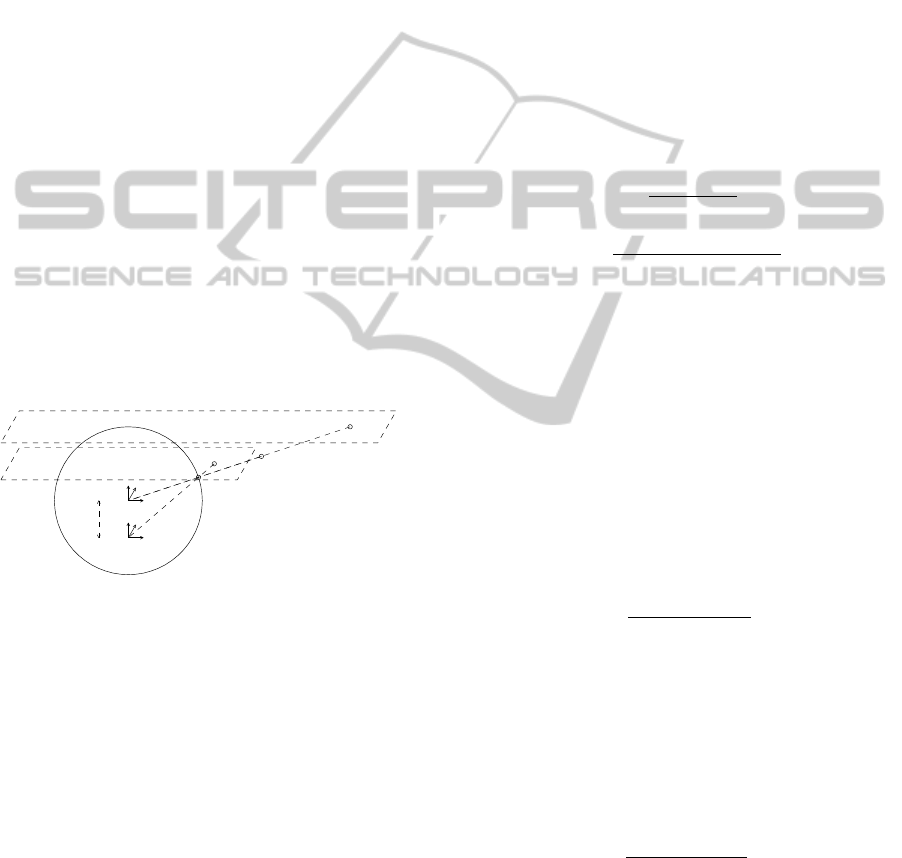
Figure 1 illustrates the spherical projection and the
perspective projection just described for the i-th gen-
eralized camera of the vision system.
F
i,s
F
i,c
X
x
i
ξ
i
X
i
Figure 1: A point X is firstly projected on the the point X
i
according to a spherical projection (frame F
i,s
). Then, the
point X
i
is projected on the image point x
i
(in normalized
coordinates) according to a perspective projection (frame
F
i,c
). The image point p
i
(in pixel coordinates) is hence
obtained as p
i
= K
i
x
i
. The distance between F
i,s
and F
i,c
is
ξ
i
, while the distance between F
i,c
and the plane where x
i
lies is 1.
Problem. The multiple-view triangulation problem
for generalized cameras consists of estimating the
scene point X from estimates of the image points
p
i
(denoted by
ˆ
p
i
) and functions Φ
i
(·) (denoted by
ˆ
Φ
i
(·)), i = 1,. .. ,N, where N is the number of gener-
alized cameras:
given
ˆ
p
i
,
ˆ
Φ
i
(·)
, i = 1, .. ., N
, estimate X. (10)
ICINCO2012-9thInternationalConferenceonInformaticsinControl,AutomationandRobotics
6
3 PROPOSED APPROACH
Let us start by observing that existing methods for tri-
angulation with perspective cameras cannot be used
to estimate X with the image points p
i
(clearly, un-
less ξ
i
= 0 for all generalized cameras, since in such
a case the cameras are perspective ones). This is due
to the fact that, as it can be seen from Figure 1, the
scene point X does not lie on the line connecting the
image point x
i
(i.e., p
i
expressed in normalized coor-
dinates instead of pixel coordinates) to the center of
its projection (i.e., F
i,c
).
The idea proposed in this paper consists of repro-
jecting the image points p
i
onto virtual image planes,
one per camera, in order to obtain new image points
for which this problem does not occur. This can be
done by determining the intersections of the lines con-
necting the scene point X to the centers of the spheri-
cal projections (i.e., F
i,s
) with virtual image planes V
i
.
Figure 2 illustrates this procedure for the i-th camera.
The virtual image plane V
i
is chosen for convenience
parallel to the true image plane of the camera and at
a unitary distance from the center of F
i,s
. The new
image point is denoted by y
i
. Let us observe that y
i
exists whenever X has a positive depth in the frame
F
i,s
, while y
i
tends to infinity as this depth tends to
zero.
F
i,s
F
i,c
X
x
i
ξ
i
y
i
X
i
V
i
Figure 2: The image point x
i
(in normalized coordinates) is
reprojected onto the virtual image plane V
i
, firstly, by deter-
mining the intersection X
i
of the line connecting x
i
to F
i,c
with the sphere, and secondly, by determining the intersec-
tion of the line connecting X
i
to F
i,s
with V
i
. The new image
point is denoted by y
i
.
In order to derive the expression of the new image
point y
i
on the virtual image plane V
i
, let us proceed
as follows. First, let us recover the expression of p
i
in
normalized coordinates, i.e. x
i
. This is given by
x
i
= K
−1
i
p
i
. (11)
Second, let us express x
i
as
x
i
=
u
i
v
i
1
(12)
where u
i
,v
i
∈ R. The line connecting x
i
to F
i,c
can be
parametrized with respect to the frame F
i,s
as
l
i
(α) =
αu
i
αv
i
−ξ
i
+ α
(13)
where α ∈ R. The spherical projection of X is hence
given by the intersection of l
i
with the sphere, i.e.
X
i
= l
i
(α
∗
) (14)
where α
∗
is the solution of
α
∗
:
kl
i
(α)k = 1
u
i
v
i
1− ξ
i
T
l
i
(α) > 0.
(15)
This solution is given by
α
∗
=
ξ
i
+ δ
i
1+ u
2
i
+ v
2
i
(16)
where
δ
i
=
q
1+ (1− ξ
2
i
)(u
2
i
+ v
2
i
). (17)
Then, the line connecting X
i
to F
i,s
can be
parametrized with respect to the frame F
i,s
as
m
i
(β) = βX
i
(18)
where β ∈ R. The intersection of this line with the
virtual image plane V
i
is hence given by
y
i
= m
i
(β
∗
) (19)
where β
∗
is the solution of
β
∗
: e
T
3
m
i
(β) = 1. (20)
This solution is given by
β
∗
=
1+ u
2
i
+ v
2
i
δ
i
− ξ
i
(u
2
i
+ v
2
i
)
. (21)
It is possible to verify that the overall expression of y
i
in normalized coordinates is given by
y
i
=
γ
i
u
i
γ
i
v
i
1
(22)
where γ
i
is defined as
γ
i
=
1+ ξ
i
δ
i
1− ξ
2
i
(u
2
i
+ v
2
i
)
. (23)
We denote the expression of y
i
as a function of p
i
ac-
cording to
y
i
= Ω
i
(p
i
). (24)
Let us observe that y
i
exists whenever
ξ
2
i
(u
2
i
+ v
2
i
) 6= 1 (25)
OntheMultiple-viewTriangulationProblemwithPerspectiveandNon-perspectiveCameras-AVirtual
Reprojection-basedApproach
7

i.e. whenever X has a positive depth in the frame F
i,s
.
The procedure just described assumes that p
i
and
Ω
i
(·) are known. However, in real situations this is
clearly not true due to the presence of uncertainties,
and hence the new image points have to be defined
using the available data. In particular, p
i
is replaced
by
ˆ
p
i
, while Ω
i
(·) is replaced by
ˆ
Ω
i
(·) which is ob-
tained as in (22)–(24) by replacing u
i
, v
i
, γ
i
, δ
i
and ξ
i
with their available estimates ˆu
i
, ˆv
i
,
ˆ
γ
i
,
ˆ
δ
i
and
ˆ
ξ
i
, re-
spectively. The estimates of the new image points are
given by
ˆy
i
=
ˆ
Ω
i
(
ˆ
p
i
). (26)
In order to estimate the scene point X, let us ob-
serve that the new image points satisfy the relation-
ship
λ
i
y
i
= P
i
X (27)
where λ
i
∈ R and P
i
∈ R
3×4
is the projection matrix
given by
P
i
=
R
i
t
i
(28)
where the rotation matrix R
i
∈ SO(3) and the transla-
tion vector t
i
∈ R
3
are given by
R
i
= O
T
i
t
i
= −O
T
i
c
i
.
(29)
Hence, (27) can be rewritten as
y
i
=
1
e
T
3
P
i
X
P
i
X. (30)
The relationship (30) can be exploited to estimate X
from the available estimates of the new image points
ˆy
i
. In the sequel we discuss two criteria for this esti-
mation.
The first method that we consider is based on the
estimation of X by minimizing the algebraic error in
the relationship (30). Specifically, according to this
method, the estimate of X is obtained through the lin-
ear least-squares problem
min
Y
ˆc
alg
(Y) (31)
where Y ∈ R
3
and
ˆc
alg
(Y) =
N
∑
i=1
e
T
1
ˆ
P
i
Y−
ˆ
γ
i
ˆu
i
e
T
3
ˆ
P
i
Y
e
T
2
ˆ
P
i
Y−
ˆ
γ
i
ˆv
i
e
T
3
ˆ
P
i
Y
!
2
(32)
and
ˆ
P
i
is the available estimate of P
i
. The solution of
linear least-squares problems can be obtained either
in closed form or through a singular value decompo-
sition (SVD). Indeed, let us define
ˆ
A =
e
T
1
ˆ
R
1
e
T
2
ˆ
R
1
.
.
.
e
T
N
ˆ
R
N
e
T
N
ˆ
R
N
,
ˆ
b =
ˆ
γ
1
ˆu
1
e
T
3
ˆ
t
1
ˆ
γ
1
ˆv
1
e
T
3
ˆ
t
1
.
.
.
ˆ
γ
N
ˆu
N
e
T
3
ˆ
t
N
ˆ
γ
N
ˆv
N
e
T
3
ˆ
t
N
. (33)
It follows that (31) can be rewritten as
min
Y
ˆ
AY−
ˆ
b
2
. (34)
The minimizer of (34), denoted by
ˆ
X
alg
, is given by
ˆ
X
alg
=
ˆ
A
T
ˆ
A
−1
ˆ
A
T
ˆ
b. (35)
Alternatively, one can get this minimizer by introduc-
ing the SVD
ˆ
U
ˆ
S
ˆ
V
T
=
ˆ
A −
ˆ
b
(36)
and by defining
ˆ
X
alg
=
ˆv
a
ˆv
b
(37)
where ˆv
a
∈ R
3
is the vector with the first three entries
of the last column of
ˆ
V ∈ R
4
and ˆv
b
∈ R is the fourth
entry of such a column.
The second method that we consider is based on
the estimation of X by minimizing the L2 norm of
the reprojection error in the relationship (30). Specif-
ically, according to this method, the estimate of X is
obtained through the optimization problem
min
Y
ˆc
L2
(Y) (38)
where
ˆc
L2
(Y) =
N
∑
i=1
e
T
1
ˆ
Ψ
i
(Y) −
ˆ
γ
i
ˆu
i
e
T
2
ˆ
Ψ
i
(Y) −
ˆ
γ
i
ˆv
i
!
2
(39)
and the function
ˆ
Ψ
i
(·) is the available estimate of the
function Ψ
i
(·) which defines the solution for y
i
in (30)
as a function of X, i.e.
y
i
= Ψ
i
(X). (40)
We denote the minimizer of (38) as
ˆ
X
L2
= argmin
Y
ˆc
L2
(Y). (41)
The computation of this minimizer can be addressed
in various ways. For instance, in (Chesi and Hung,
2011) a technique based on convex programming has
been proposed recently,which provides a candidate of
the sought solution and a simple test for establishing
its optimality. See also the other techniques described
in the introduction.
It is important to observe that the two methods just
described provide estimates of the sought scene point
by minimizing an error (either algebraic or geomet-
ric) defined for the new image points ˆy
i
. This means
that such an error is evaluated on the virtual image
planes V
i
unless the cameras are perspective (in such
a case, in fact, the virtual image planes V
i
coincide
with the image planes of the cameras). Let us also
ICINCO2012-9thInternationalConferenceonInformaticsinControl,AutomationandRobotics
8
observe that the estimates provided by these methods
approach the sought scene point as image noise and
calibration errors tend to zero (clearly, if enough in-
formation is available for triangulation).
In the sequel we denote the 3D estimation errors
achieved by minimizing the algebraic error in (31)
and by minimizing the L2 norm of the reprojection
error in (38) as
d
alg
= k
ˆ
X
alg
− Xk
d
L2
= k
ˆ
X
L2
− Xk .
(42)
4 EXAMPLES
In this section we present some results obtained with
synthetic and real data. The minimization of the al-
gebraic error in (31) is solved through (35), while
the minimization of the L2 norm of the reprojec-
tion error in (38) is solved with the TFML method
described in (Chesi and Hung, 2011) available at
http://www.eee.hku.hk/∼chesi. In both cases, the
data are pre-elaborated in order to work with normal-
ized data.
4.1 Example 1
Let us consider a vision system composed by three
generalized cameras with 180 degrees-field of view
defined by
∀i = 1, 2,3
K
i
=
200 0 400
0 200 400
0 0 1
ξ
i
= 0.5
O
i
= e
[θ
i
]
×
and
θ
1
=
0
0
0
, c
1
=
−9
4
1
θ
2
=
−π/2
0
0
, c
2
=
3
−1
−7
θ
3
=
0
−π/3
π/2
, c
3
=
1
7
6
.
The scene point is
X =
1
2
3
and the corresponding image points in pixel coordi-
nates are given by
p
1
=
677.926
344.415
1
, p
2
=
351.895
159.473
1
p
3
=
133.527
465.346
1
.
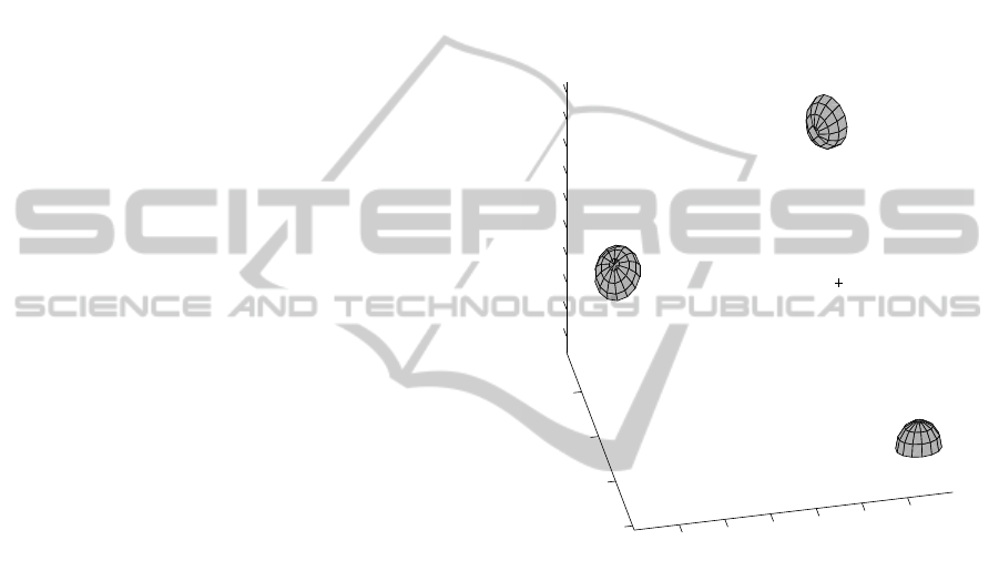
Figure 3 shows the three cameras and the scene point,
while Figures 4a–4c show the image points and the
boundary of the visible region in each camera.
−8
−6
−4
−2
0
2
−10
−5
0
5
−1
0
1
2
3
4
5
6
7
8
x
y
z
Figure 3: Example 1: the three cameras and the scene point
(“+” mark).
In this example we want to consider the presence
of image noise on the available image points. To this
end, we define the available image points as
ˆ
p
i
= p
i
+ ηn
i
∀i = 1, 2,3
where η is a parameter defining the image noise in-
tensity and
n
1
=
1
1
0
, n
2
=
1
−1
0
, n
3
=
−1
1
0
.
The problem consists of estimating X for η varying in
the interval [0,6] pixels.
We repeat the multiple-view triangulation proce-
dure described in the previous section for a grid of
values η in [0,6]. Figure 5 shows the obtained esti-
mates by minimizing the algebraic error and by mini-
mizing the L2 norm of the reprojection error. In par-
ticular, for η = 6, the 3D estimation errors achieved
OntheMultiple-viewTriangulationProblemwithPerspectiveandNon-perspectiveCameras-AVirtual
Reprojection-basedApproach
9
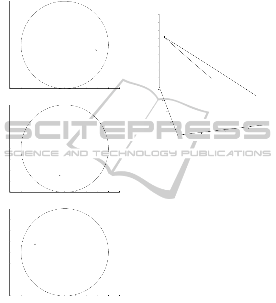
−100 0 100 200 300 400 500 600 700 800 900
100
200
300
400
500
600
700
[pixel]
[pixel]
(a)
−100 0 100 200 300 400 500 600 700 800 900
100
200
300
400
500
600
700
[pixel]
[pixel]
(b)
−100 0 100 200 300 400 500 600 700 800 900
100
200
300
400
500
600
700
[pixel]
[pixel]
(c)
Figure 4: Example 1: image points (“o” marks) and bound-
ary of the visible region (solid line) for each camera.
by the two methods are
d
alg
= 0.231, d
L2
= 0.139.
As we can see, minimizing the algebraic error pro-
vides quite worse estimates than minimizing the L2
norm of the reprojection error in this example. Inter-
esting, the next examples will show that the situation
is generally different.
1
1.05
1.1
1.15
2.85
2.9
2.95
3
3.05
1.86
1.88
1.9
1.92
1.94
1.96
1.98
2
2.02
x
y
z
ˆ
X
alg
ˆ
X
L2
Figure 5: Example 1: solutions
ˆ
X
alg
and
ˆ
X
L2
for η ∈ [0, 6].
4.2 Example 2: Statistics with Synthetic
Data
Here we present some results obtained with synthetic
data. Specifically, we have generated 500 vision sys-
tems, each of them composed by a scene point to re-
construct (denoted hereafter as X) and 4 generalized
cameras with 180 degrees-field of view, in particular
with intrinsic parameters given by
∀i = 1,..., 4
K
i
=
300 0 600
0 200 400
0 0 1
ξ
i
= 0.5.
For each vision system, X and the centers of the cam-
eras are randomly chosen in a sphere of radius 500
centered in the origin of the reference frame, while the
orientation matrices of the cameras are randomly cho-
sen under the constraint that X is visible by the cam-
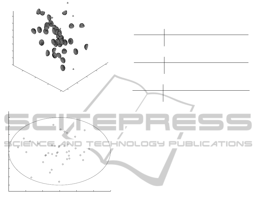
eras. Figure 6a shows the scene points and the gener-
alized cameras for 10 of the 500 vision systems, while
Figure 6b shows the image points and the boundary of
the visible region in these cameras.
In order to generate the corrupted data, we have:
• added random variables in the interval [−η,η]
pixels to each coordinate of the image points,
where η ∈ R defines the noise intensity;
• multiplied ξ and each intrinsic parameter times
random variables in the interval [1 − η/100,1+
η/100];
ICINCO2012-9thInternationalConferenceonInformaticsinControl,AutomationandRobotics
10
−50
0
50
100
−100
−50
0
50
100
−80
−60
−40
−20
0
20
40
60
x
y
z
(a)
0 200 400 600 800 1000 1200
0
100
200
300
400
500
600
700
800
[pixel]
[pixel]
(b)
Figure 6: Example 2 (synthetic data): (a) scene points (“+”
marks) and generalized cameras for 10 of the 500 vision
systems; (b) image projections of such scene points (“o”
marks) and boundary of the visible region (solid line).
• multiplied the camera centers and the angles of
the rotation matrices times random variables in
the interval [1− η/100,1+ η/100].
Hence, we have repeated the triangulation for 3
numbers of available cameras (i.e., 2, 3 and 4) and
for 4 values of noise intensity (i.e., η = 0.5,1,1.5,2),
hence solving a total number of 3 × 4 × 500 = 6000
triangulation problems. Table 1 shows the average
values of d
alg
and d
L2
denoted by “alg” and “L2”, re-
spectively.
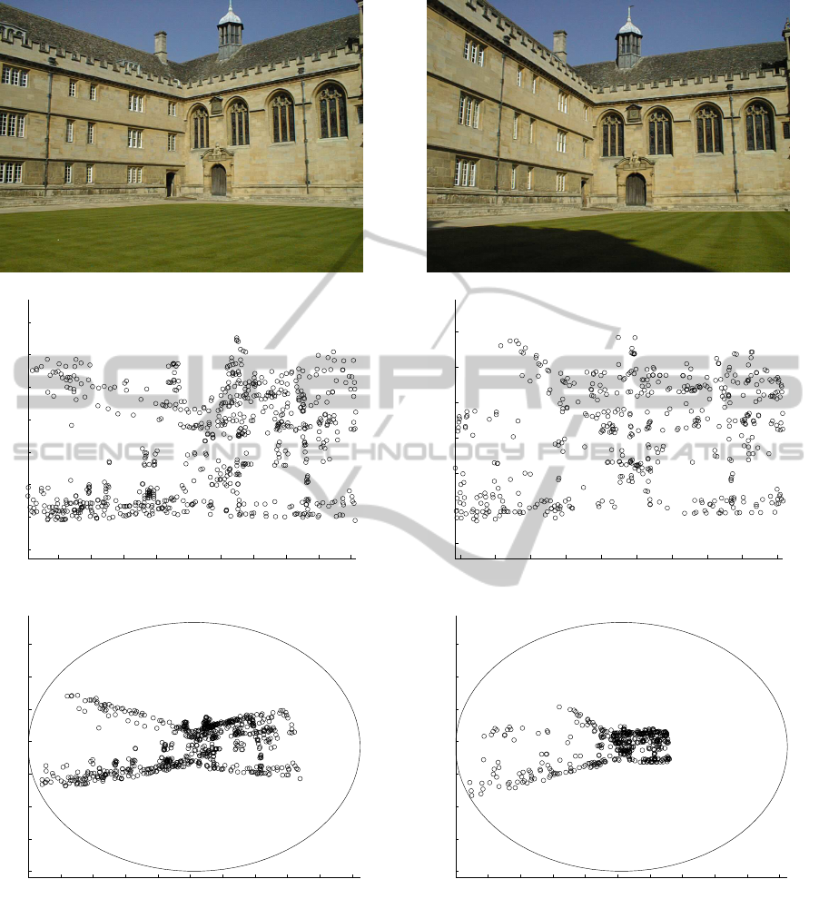
4.3 Example 3: Wadham College
Sequence
Lastly, we present some results obtained with almost
real data. In fact, we do not have real data for a non-
perspective camera, moreover with real data it is im-
Table 1: Example 2 (synthetic data): average 3D error for
different number of generalized cameras (N) and noise in-
tensity (η).
N = 2 (2000 points)
method \ η 0.5 1 1.5 2
alg 2.021 3.6212 6.1174 8.1519
L2 2.0181 4.0248 6.1692 8.42
N = 3 (2000 points)
method \ η 0.5 1 1.5 2
alg 1.0846 2.1688 3.0144 4.1615
L2 1.0817 2.0342 3.047 4.2966
N = 4 (2000 points)
method \ η 0.5 1 1.5 2
alg 0.9066 1.7793 2.4941 3.4809
L2 0.94721 1.7375 2.5739 3.8066
possible to know the true scene points that we would
like to use for evaluation. Hence, we have considered
the Wadham college sequence available at the web-
page of the Visual Geometry Group of Oxford Uni-
versity, http://www.robots. ox.ac.uk/∼vgg/data/data-
mview.html. This sequence consists of 5 views taken
with a perspective camera, the projection matrices of
such views, and 3019 image points corresponding to
1331 scene points visible in at least 2 of such views
(with known correspondence).
In particular:
• 1052 points are visible in 2 views;
• 215 points are visible in 3 views;
• 50 points are visible in 4 views;
• 14 points are visible in 5 views.
First, we have estimated the 1331 scene points using
standard triangulation for perspective cameras, which
are shown in Figure 9. Second, we have computed
the projections of these scene points onto generalized
cameras with same orientation, same center except
for a translation along the optical axis in order to en-
large the spanned image area, and intrinsic parameters
given by
∀i = 1,..., 5
K
i
=
256 0 512
0 192 384
0 0 1
ξ
i
= 0.5.
Figures 7–8 show the first image and last one of
the 5 images, the corresponding extracted points, and
the same points after transforming and shifting the
cameras.
The data obtained so far will be used as “true”
data. Third, we have corrupted the true data as done in
the previous subsection for the case of synthetic data
with noise intensity η = 1. Fourth, we have repeated
OntheMultiple-viewTriangulationProblemwithPerspectiveandNon-perspectiveCameras-AVirtual
Reprojection-basedApproach
11
(a)
100 200 300 400 500 600 700 800 900 1000
100
200
300
400
500
600
700
800
[pixel]
[pixel]
(b)
0 100 200 300 400 500 600 700 800 900 1000
0
100
200
300
400
500
600
700
[pixel]
[pixel]
(c)
Figure 7: Example 3 (Wadham college sequence): (a) first
image of the sequence; (b) points extracted in such an im-
age; (c) same points after transforming and shifting the
cameras.
the triangulation using for each scene point the max-
imum number of cameras where the point is visible.
Table 2 shows the average values of d
alg
and d
L2
de-
noted by “alg” and “L2”, respectively.
(a)
100 200 300 400 500 600 700 800 900 1000
100
200
300
400
500
600
700
[pixel]
[pixel]
(b)
0 100 200 300 400 500 600 700 800 900 1000
0
100
200
300
400
500
600
700
[pixel]
[pixel]
(c)
Figure 8: Example 3 (Wadham college sequence): (a) last
image of the sequence; (b) points extracted in such an im-
age; (c) same points after transforming and shifting the
cameras.
5 CONCLUSIONS
We have addressed the multiple-view triangulation
problem in a vision system with perspective and
ICINCO2012-9thInternationalConferenceonInformaticsinControl,AutomationandRobotics
12

−16
−14
−12
−10
−8
−6
−4
−2
0
2
−15
−10
−5
0
5
10
0
5
10
15
20
x
y
z
Figure 9: Example 3 (Wadham college sequence): esti-
mated scene points.
Table 2: Example 3 (Wadham college sequence): average
3D error for different number of generalized cameras (N).
N alg L2
2 6.2038 8.4202
3 1.2768 1.3405
4 1.0436 0.93116
5 0.34739 0.3462
non-perspective cameras, and we have proposed an
approach based on reprojecting the available image
points onto virtual image planes. This approach has
the advantage of transforming the original problem
into a new one for which the existing methods for
multiple-view triangulation with perspective cameras
can be used. In particular, algebraic and geometric er-
rors of such methods are now evaluated on the virtual
image planes, and the solution of the new problem
exactly approaches the sought scene point as image
noise and calibration errors tend to zero.
The obtained numerical results suggest that mini-
mizing the simple algebraic error on the virtual image
planes can provide competitive estimates compared
with those provided by the minimization of the L2
norm of the reprojection error on such planes. This is
indeed interesting, and it is probably due to the dif-
ferent meaning that the L2 norm assumes when eval-
uated for the new image points. Future work will in-
vestigate this aspect.
REFERENCES
Byrod, M., Josephson, K., and Astrom, K. (2007). Fast
optimal three view triangulation. In Asian Conf. on
Computer Vision, volume 4844 of LNCS, pages 549–
559, Tokyo, Japan.
Chesi, G. and Hung, Y. S. (2007). Global path-planning for
constrained and optimal visual servoing. IEEE Trans.
on Robotics, 23(5):1050–1060.
Chesi, G. and Hung, Y. S. (2011). Fast multiple-view L2 tri-
angulation with occlusion handling. Computer Vision
and Image Understanding, 115(2):211–223.
Chesi, G. and Vicino, A. (2004). Visual servoing for
large camera displacements. IEEE Trans. on Robotics,
20(4):724–735.
Faugeras, O. and Luong, Q.-T. (2001). The Geometry of
Multiple Images. MIT Press, Cambridge (Mass.).
Hartley, R. and Schaffalitzky, F. (2004). l
∞
minimization
in geometric reconstruction problems. In IEEE Conf.
on Computer Vision and Pattern Recognition, pages
504–509, Washington, USA.
Hartley, R. and Sturm, P. (1997). Triangulation. Computer
Vision and Image Understanding, 68(2):146–157.
Hartley, R. and Zisserman, A. (2000). Multiple view in com-
puter vision. Cambridge University Press.
Lu, F. and Hartley, R. (2007). A fast optimal algorithm for
l
2
triangulation. In Asian Conf. on Computer Vision,
volume 4844 of LNCS, pages 279–288, Tokyo, Japan.
Stewenius, H., Schaffalitzky, F., and Nister, D. (2005). How
hard is 3-view triangulation really? In Int. Conf. on
Computer Vision, pages 686–693, Beijing, China.
OntheMultiple-viewTriangulationProblemwithPerspectiveandNon-perspectiveCameras-AVirtual
Reprojection-basedApproach
13
