Modeling Dynamic Systems for Diagnosis
PEPA/TOM4D Comparison
I. Fakhfakh
1
, M. Le Goc
2
, L. Torres
2
and C. Curt
1
1
IRSTEA, 3275 route de C
´
ezanne - CS 40061, Aix-en-Provence, France
2
Aix-Marseille Univ, LSIS, 13397 Marseille, France
Keywords:
Multi Modeling, Model Based-reasoning, Dynamic System, Process Algebras, Timed Observation Theory.
Abstract:
Researchers have long been seeking the most suitable formalism and method to build models of dynamic
systems for diagnostic tasks. In this paper, we claim that the main difficulty stems from the lack of global
formalism capable of taking into account structural, functional and behavioral knowledge. To illustrate this
point, we propose a comparison between two modeling approaches.
1 INTRODUCTION
In the last two decades model-based diagnosis has
been an important area of research in which numerous
new methodologies and formalisms have been pro-
posed, studied and subjected to experiments (Con-
sole et al., 2000) and (Le Goc et al., 2008). This
is motivated by the practical need for ensuring the
correct and safe operation of large complex systems.
Since (Reiter, 1987), most of frameworks have been
based on logic formalism. Despite major contribu-
tions in the domain of temporal logic, a difficulty re-
mains in taking observation time into account in di-
agnosis reasoning. Therefore many works have been
proposed to define more or less specific formalisms
to overcome this limit to the logical representation
of timed knowledge, such as the discrete event sys-
tem (D.E.S) formalism and the multi-modeling ap-
proach of (Chittaro et al., 1993). Moreover, these
approaches have seldom been used in the context of
diagnosis. More recently, PEPA formalism (Perfor-
mance Evaluation Process Algebra) (Console et al.,
2000) and the TOM4D methodology (Timed Obser-
vation Modeling for Diagnosis) (Le Goc et al., 2008)
have been proposed to provide expressive languages
to enable efficient modeling of dynamic systems for
diagnosis, comprising a component centered model-
ing paradigm.
The goal of this paper is to bridge research into
process algebras and timed observation modeling
(Le Goc et al., 2008) by providing a comparison be-
tween PEPA and TOM4D. This comparison is per-
formed with a concrete example(Section 2).
2 A HYDRAULIC SYSTEM
The dynamic system studied in (Console et al., 2000)
is described in Figure 1. We use this example to com-
pare PEPA and TOM4D.
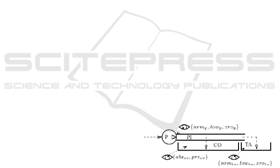
Figure 1: Hydraulic system of (Console et al., 2000).
” The system is formed by a pump P which deliv-
ers water to a tank TA via a pipe PI; another tank CO
is used as a collector for water that may leak from the
pipe. For the sake of simplicity, we assume that the
pump is always on and supplied with water. Pump P
has three modes of behavior: OK (the pump produces
a normal output flow), leaking (it produces a low out-
put flow), and blocked (no output flow). Pipe PI can
be OK (delivering the water it receives from the pump
to the tank) or leaking (in this case we assume that
it delivers a low output to the tank a when receiving
a normal or low input, and no output when receiving
no input). Tanks TA and CO are always in OK mode,
i.e., they simply receive water. We assume that three
sensors are available (see the eyes in Figure 1): flowp
measures the flow from the pump, which can be nor-
mal (nrm
p
), low (low
p
), or zero (zro
p
); level
TA
mea-
sures the level of the water in TA, which can be normal
(m
ta
), low (low
ta
), or zero (zro
ta
); level
co
records the
183
Fakhfakh I., Le Goc M., Torres L. and Curt C..
Modeling Dynamic Systems for Diagnosis - PEPA/TOM4D Comparison.
DOI: 10.5220/0003987201830186
In Proceedings of the 14th International Conference on Enterprise Information Systems (ICEIS-2012), pages 183-186
ISBN: 978-989-8565-10-5
Copyright
c
2012 SCITEPRESS (Science and Technology Publications, Lda.)
presence of water in CO, which can be either present
(pre
co
) or absent (abs
co
)”.
3 PEPA MODEL
The PEPA model is based on classical process alge-
bras enhanced with timed information. Process al-
gebras are abstract languages based on a component
oriented approach (Console et al., 2000) where each
component is modeled in isolation and then each of
the models of the components is composed using the
operators provided by the calculation in order to ob-
tain the entire model. In PEPA, the model of a physi-
cal system is usually divided into two parts: A behav-
ioral model(BM) and a structural model(SM).
3.1 Structural Model
SM describes the structure of the system in terms of
its components. Each component is represented as an
instantiation of generic model. In the example stud-
ied (cf. Figure 1), four generic behaviors are defined:
the ”P” behavior (Pump), the ”PI” behavior (Pipe),
the ”TA” behavior (TA tank) and the ”CO” behavior
(CO tank); also four component instances can be de-
clared: P
(1)
: P; PI
(1)
: PI; TA
(1)
: TA; CO
(1)
: CO.
P
(1)
: P means that the component P
(1)
is an instance
of a component whose behavior is P. The connection
between them is ensured by the cooperation operator
L
i
where the sets L
i
define the activities on which the
components must cooperate. Equation SD
1
describes
the SM of the hydraulic system. The SM of the exam-
ple is:
SD
1
de f
= (P
(1)
L
1
∪{end}
(PI
(1)
L
2
∪{end}
(TA
(1)
{end}
CO
(1)
) )
where L
1
= {nrm
p
, low
p
, zro
p
}, L
2
= {nrm
1
, low
1
,
zro
1
, abs
2
, pre
2
}, H = {nrm
0
, nrm
1
, low
1
, zro
1
, abs
2
,
pre
2
}. The TA
(1)
tank, for example, cooperates with
the CO
(1)
tank with the ”end”
3.2 Behaviour Model
The behavior of each component type is described
as a nondeterministic choice between the various
modes. For example, the BM of the pipe is the
following: PI = PIok
1
+ PIlk
1
+ End;
PIok
1
= nrm
p
.PIok
2
+ low
p
.PIok
3
+ zro
p
.PIok
4
;
PIok
2
= nrm
1
.abs
2
.PI ;
PIok
3
= low
1
.abs
2
.PI;
PIok
4
= zro
1
.abs
2
.PI;
PIlk
1
= nrm
p
.PIlk
2
+ low
p
.PIlk
2
+ zro
p
.PIlk
3
;
PIlk
2
=low
1
.pre
2
.PI; PIlk
3
= zro
1
.abs
2
.PI;
End = end.End
For each behavior, a set of equations is defined
to specify the relations between the component vari-
ables. In particular, the actions of PEPA are used
to express conditions on input, output and state vari-
ables. PI = PIok
1
+ PIlk
1
+ End means that the com-
ponent PI may either be in OK behavior (PIok
1
) or
in leaking behavior (PIlk
1
). The additional identifier
End allows the component to evolve into a final state.
4 TOM4D MODEL
TOM4D is a multi-model approach that combines
CommonKads templates with the conceptual frame-
work proposed in (Zanni et al., 2006) and the tetrahe-
dron of states (T.O.S), (Chittaro et al., 1993). These
elements are merged according to the Timed Obser-
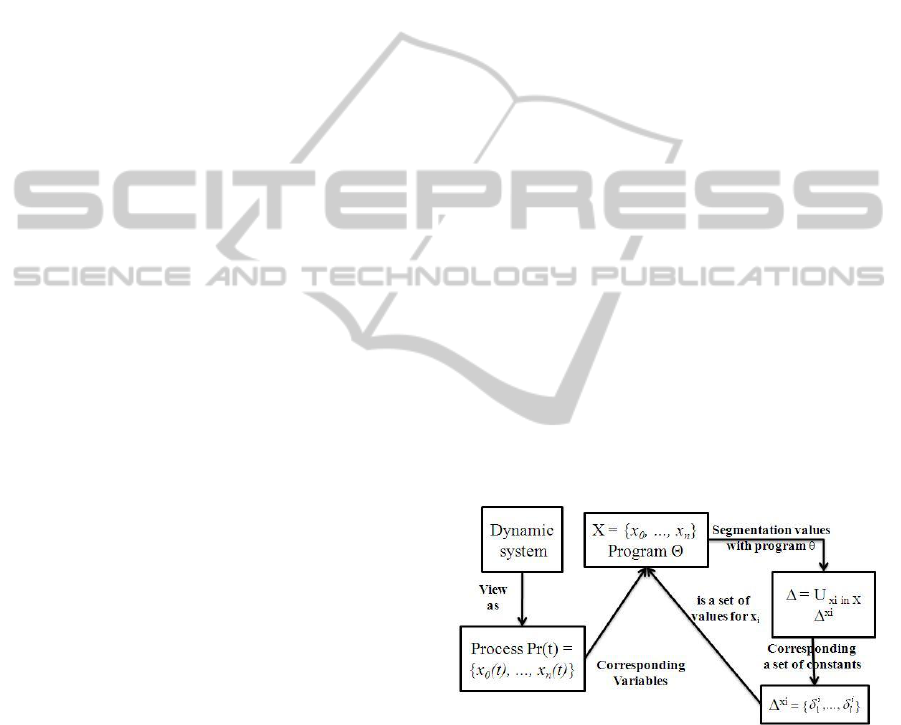
vations Theory (cf Figure 2 more details in (Le Goc,
2006)). In this theory, it is usual to define an observa-
tion class C
i
={(x
i
, δ
i
j
)} as a singleton to associate one
variable x
i
with a constant δ
i
j
. The concept of obser-
vation class is close to the notion of discrete event in
the D.E.S domain. Figure 3 describes the three main
steps of the TOM4D modeling process: The Knowl-
edge Interpretation step uses a CommonKADS tem-
plate to interpret and organize available knowledge
(an expert, a set of documents, etc.) of a dynamic
system.
Figure 2: Timed Observation Theory: abstract.
The scenario model M(ω)= < SM(ω), FM(ω),
BM(ω)> of the system is consistent with knowledge
available on its evolution over time. This model
is necessary to provide, by using the tetrahedron of
states, a physical and a logical interpretation of the
terms used (variables, constants, etc.). In the exam-
ple studied two physical dimensions are given for the
variables: volume (m
3
) and flows of water (m
3
.s
−1
)
(leaking and normal output). This leads to using the
Hydraulic T.O.S. where no pressure (Pr), no resistiv-
ity (R) or pressure moment (Pp) are evoked in the
ICEIS2012-14thInternationalConferenceonEnterpriseInformationSystems
184
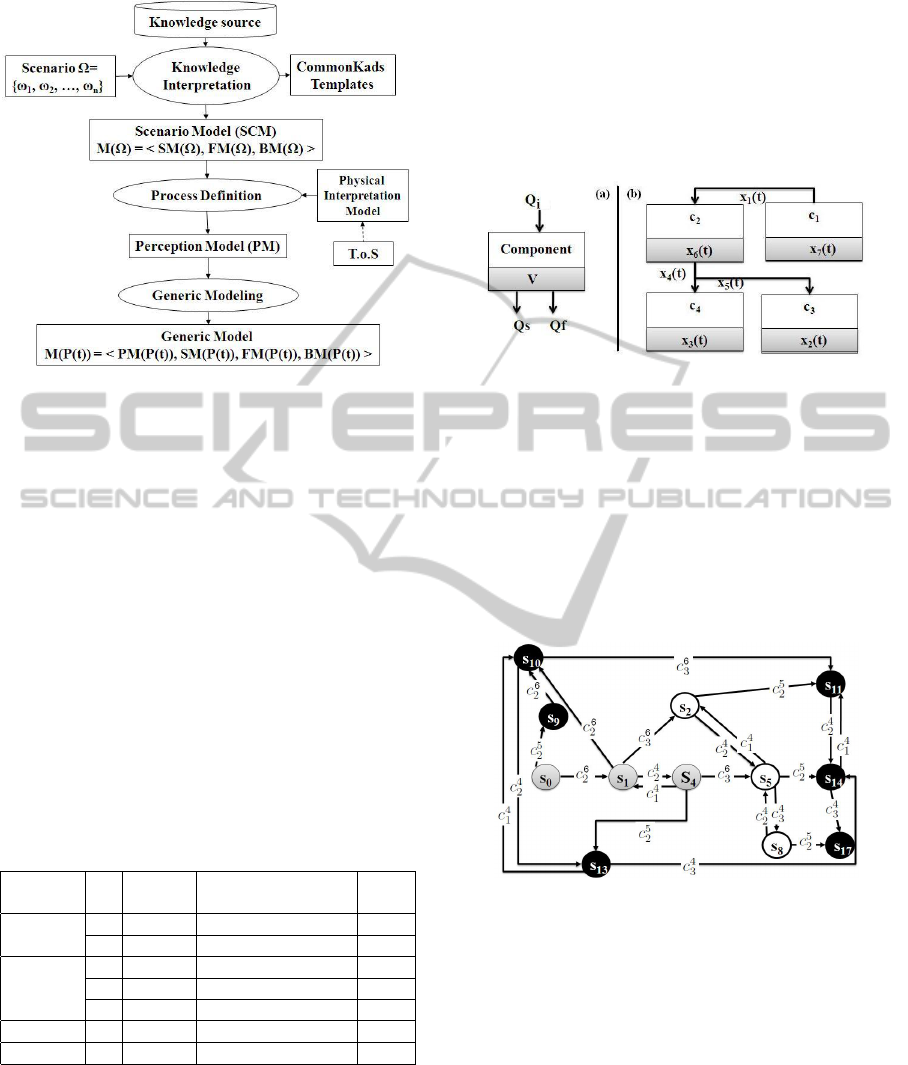
Figure 3: TOM4D Modeling Process.
available knowledge. Thus it is easy to design an ab-
stract generic hydraulic component forming a relation
between an input flow Qi(t), an internal volume V (t)
and two output flows, a normal output flow Qs(t) and
an uncontrolled output flow Q f (t) (Figure 4a). Such a
component is generic because it can be used to model
all the components of the system.
4.1 Perception Model: PM
The abstract generic hydraulic component is sufficient
to define the role of each variable of the system and
the associated concrete components.
Table 1 shows the component-variable-value as-
sociation that can be made according to the abstract
generic hydraulic component.
Table 1: component-variable-value association.
COMPS X dimen- Action ∆
sion (PEPA)
c
1
x
7
V nrm
0
, low
0
,zro
0
2,1,0
x
1
Qs nrm
p
,low
p
,zro
p
2,1,0
c
2
x
6
V nrm
pi
,low
pi
,zro
pi
2,1,0
x
4
Qs nrm
1
,low
1
,zro
1
2,1,0
x
5
Q f pres
2
,abs
2
1,2
c
3
x
2
V nrm
TA
low
TA
,zro
TA
2,1,0
c
4
x
3
V pres
CO
, abs
CO
1,2
4.2 Structural Model
A TOM4D structural model SM(P(t)) is a 3-tuple <
COMPS, R
p
, R
x
> (cf. Figure 4) where:
• COMPS={c
1
, c
2
, c
3
, c
4
} is the finite set of con-
stants denoting the system components,
• R
p
is a set of equality predicates defin-
ing the interconnections between the compo-
nents. R
p
={out(c
1
)=in(c
2
), out
1
(c
2
)=in(c
3
),
out
2
(c
2
)=in(c
4
)}
• R
x
is a set of equality predicates linking each vari-
able. R
x
={ out(c
1
)=x
1
, out(c
3
)=x
2
, out(c
4
)=x
3
,
out
1
(c
2
)=x
4
, out
2
(c
2
)=x
5
}.
Figure 4: Structural Model SM(P(t)).
4.3 Behavioral Model
The behavior model BM(P(t)) is a 3-tuple < S,C, γ >
where S = {s
i
}
i=1...l
is a set of states (s
0
for example
corresponds on x
6
=0 ∧ x
4
=0 ∧ x
5
=1), C is a set of
timed observation classes C
i
={(x
i
, δ
i
j
} (C
6
1
= {(x
6
,0)}
for example) and γ: S × C → S is the state transi-
tion function that implements the state evolution in
the system modeled (i.e. γ(s
1
,C
6
3
) = s
2
).
Figure 5: Behavioral Model of the Pipe.
The ok and leaking PEPA modes of the pipe cor-
respond to the grey and black states in Figure 5, re-
spectively.
4.4 Functional Model: FM
A functional model FM is a 3-tuple < ∆, F, R
f
>
where ∆ is the set of values assumable by the differ-
ent variables (∆
x
1
= {2, 1, 0} for example), F is a set of
functions (The result of the T.o.S and structural model
denotes 7 functions ) and R
f
is a set of equality pred-
icates defining a variable as a function of the others.
The graph of FM(P(t)) is shown in figure 6).
ModelingDynamicSystemsforDiagnosis-PEPA/TOM4DComparison
185

Figure 6: Functional Model of the hydraulic system.
5 DISCUSSION AND
CONCLUSIONS
The example studied shows that the TOM4D struc-
tural model plays the same role as the declaration of
generic component instances, the connection equa-
tions and the activities declaration in PEPA formal-
ism.
The functional TOM4D models play the same role
as the so called ”behavioral” model of components in
Reiter’s theory. There is no equivalent in PEPA be-
cause the process algebras are centered with the de-
scription of the behavioral properties of the connected
components. In this perspective, the value of a vari-
able at a particular time depends on the different ac-
tivities at work in the process. Consequently, the FM
cannot be modelled in the modeling process.
Process algebras define the set of states through
a set of symbols corresponding to an expert’s lan-
guage items, contrary to TOM4D where the states
are anonymous: their meanings are provided with the
value of the whole set of variables used when the sys-
tem enters a state. The set of PEPA actions plays the
same role as the set of timed observation classes and
the behavior definition is similar to the set of transi-
tion relations of the TOM4D behavioral models. Such
a behavioral model is not covered by Reiter’s theory.
In other words, a diagnosis model built according to
Reiter’s theory is formulated with a structural model
and a functional model in the TOM4D meaning. A di-
agnosis model built according to PEPA is formulated
with a structural model and a behavioral model.
On the other hand, the TOM4D methodology
obliges the experts to define the way they ”see” the
system in order to model in terms of perception.
There is no equivalent in PEPA because it consid-
ers the diagnosis model as a consequence of both the
system structure and the behavior of its components.
This was one of the reason for proposing TOM4D.
An important property of the TOM4D methodol-
ogy is the use of T.O.S. T.O.S. facilitates the introduc-
tion of a physical interpretation to model behaviors
having a physical meaning.
From the technical viewpoint, the PEPA model is
more compact than TOM4D models. A compact rep-
resentation is an advantage for the modeler since the
lower the number of symbols there are to be defined,
the better the model will be.
One the advantages of TOM4D is precisely that
its makes explicit the different relations between the
terms used by an expert to formulate their knowledge
(variable, value, state transition condition, etc). In
other words, TOM4D obliges experts to clarify their
knowledge when analyzing the system to be modeled
according to four points of view: perception, struc-
ture, function and behavior. From this standpoint,
the graphical representations of TOM4D models are
clearly an advantage for interpreting and validating
them.
Finally, TOM4D methodology provides concepts
and tools to help the modeler to define the correct
level of abstraction for efficient diagnosis. The ex-
periments we performed with TOM4D methodology
show that this level of abstraction corresponds to that
used by an expert to formulate their knowledge of di-
agnoses applied to dynamic systems.
We are now investigating these approaches to
characterize the properties of their diagnosis algo-
rithms (computational and pertinence properties).
ACKNOWLEDGEMENTS
The authors would like to thank the PACA region and
FEDER for their funding.
REFERENCES
Chittaro, L., Guida, G., Tasso, C., and Toppano, E. (1993).
Functional and teological knowledge in the multi-
modeling approach for reasoning about physical sys-
tems: A case study in diagnosis. IEEE Transactions
on Systems, Man, and Cybernetics 23(6), 1718-1751.
Console, L., Picardi, C., and Ribaudo, M. (2000). Diag-
nosing and diagnosability analysis using pepa. Paper
presented at the 14th European Conference on AI.
Le Goc, M. (2006). Notion d’observation pour le diagnostic
des processus dynamiques : application Sachem et la
dcouverte de connaissances temporelles. Universit
´
e
Aix-Marseille III - FST.
Le Goc, M., Masse, E., and Curt, C. (2008). Modeling pro-
cesses from timed observations. (ICSoft 2008).
Zanni, C., Le Goc, M., and Frydmann, C. (2006). A con-
ceptual framework for the analysis, classification and
choice of knowledge-based system. In International
Journal of Knowledge-based and Intelligent Engi-
neering Systems, 10, pages 113–138. Kluwer Aca-
demic Publishers.
ICEIS2012-14thInternationalConferenceonEnterpriseInformationSystems
186
