Design of Human-computer Interfaces in Scheduling Applications

Anna Prenzel and Georg Ringwelski

Hochschule Zittau / Görlitz, Department of Electrical Engineering and Computer Science,

Obermarkt 17, 02826, Görlitz, Germany

Keywords: Human Factors, Planning and Scheduling, Decision Support System, Automation, Interactive Scheduling.

Abstract: There are many algorithms to solve scheduling problems, but in practice the knowledge of human experts

almost always needs to be involved to get satisfiable solutions. In this paper, we describe a set of decision

support features that can be used to improve human computer interfaces for scheduling. They facilitate and

optimize human decisions at all stages of the scheduling procedure. Based on a study with 35 test subjects

and overall 105 hours of usability testing we verify that the use of the features improves both quality and

practicability of the produced schedules.

1 INTRODUCTION

Scheduling solutions to support human decisions are

widely asked for in several application domains.

Very often these solutions turn out in practice to

work as sociotechnical or mixed initiative systems.

Numerous (human) agents and stakeholders as well

as software systems are involved in decision making

(Burstein and McDermott, 1997), (Wezel et al.,

2006).

Problem Description. In this paper we focus

practical scheduling problems. A fleet scheduling

system serves as an example. It is to be included in

an information system for water suppliers. The final

product is sold to several companies, which have

similar, but never uniform problems and workflows.

The customers require interactive scheduling

features including

• adapting schedules during execution due to

accidents that must be resolved immediately

• adapting future schedules due to expert

knowledge which was not included in the model a

priori

• allowing manual adaptation in order to evaluate

different scenarios for parts of a future schedule.

Another problem is the acceptance of the product

by end-users. In interviews with human schedulers

we have observed that

• they fear that a system could replace their work

and are reluctant to accept push-the-button-

optimizers

• consequently they tend to find problems in the

produced schedules, which can hardly be solved a

priori through better modeling

• it is inevitable that expert knowledge on the

scheduling process is maintained in a company.

From this point of view we must find appropriate

ways to incorporate human factors in the computer-

supported scheduling process.

Contribution. In order to target these

requirements we define several human-computer

interaction models based on an analysis of human

decision-making. They can be distinguished by their

level of automation that varies between manual and

fully automatic.

• We deduce a set of decision support (DSS)

features from this analysis that can be combined to

different human-computer interaction models.

• We show that human operators should be able

to choose the level of automation for each

scheduling problem individually.

• We compare the models based on an empirical

study we carried out in 105 hours of usability

testing with 35 test subjects. Our study shows that

the quality of the produced schedules correlates

with use and availability of the regarded features.

219

Prenzel A. and Ringwelski G..

Design of Human-computer Interfaces in Scheduling Applications.

DOI: 10.5220/0003987402190228

In Proceedings of the 14th International Conference on Enterprise Information Systems (ICEIS-2012), pages 219-228

ISBN: 978-989-8565-10-5

 2012 SCITEPRESS (Science and Technology Publications, Lda.)

2 A SHORT INTRODUCTION

INTO PRACTICAL

SCHEDULING

2.1 The Common Structure of

Scheduling Problems

The main concern of scheduling is the assignment of

jobs to resources. Jobs are services that must be

carried out by the resources, for example, items for

production, items for transport or shifts in a hospital.

Machines, vehicles and employees can be

considered as resources. Scheduling systems are

expected to solve combinatorial problems such as

finding sequences or start times of jobs, good

resource utilization, minimal makespan and many

more. Solving these problems is complex (often NP-

complete) because solutions have to satisfy

numerous constraints including

Start Time Constraints:

For individual jobs, such as “each job has a time

window that restricts earliest and latest possible start

time”.

Among several jobs, such as “jobs must not overlap

in time if they are assigned to the same resource”.

Resource Constraints:

For individual jobs, such as “each job has a set of

resources it can be assigned to”.

Among several jobs, such as “a limited set of

resources can be used at a time”.

Our case study in fleet scheduling is based on a

formal model described by Kallehauge, Larsen,

Madsen and Solomon (2005). In addition to meeting

the constraints the goal of scheduling is to keep costs

low and to minimize the execution time. The

calculation of the costs is again application-specific.

The objective functions of our fleet scheduling

system are:

a) The total travel time between each two jobs in

the schedule (cost function)

b) The time between the beginning of the first and

the end of the last job in the schedule (execution

time)

The latter also addresses the common

requirement of balancing the workload of the

resources. Scheduling aims to find an arrangement

of jobs that optimizes the current objective values

and provides a good tradeoff between them.

2.2 Preferences and Modifications

We have gathered information about scheduling

issues in several projects with domain experts in

scheduling. Each company has its specific technical

requirements on their schedules. For example, a

manufacturing company will define the sequence, in

which items are processed on the assembly line. The

individual start time and resource constraints reflect

the physical conditions of the production system and

thus have to be enforced as hard constraints.

However, the dispatchers also know the criteria

that make their schedules practicable or

impracticable and prefer certain schedules over

others. Their preferences arise from dynamic

changes in the operational requirements. Consider

the following types of preferences:

Start Time Preferences: “start this job not until

10 o’clock”; “start this job as early as possible”

Resource Preferences: “use resource X (not) for

this job”; “use only half of the jobs for this resource”

Optimization Preferences: “reduce the travel

time for this resource”; “reduce the overall execution

time”; “change the weight of this objective function”

Preferences like these are based on the

experience of the human operators in their field of

work (Fransoo et al., 2011). They have an idea of

what an “optimal” schedule looks like in a particular

situation. This also means that they are able to find

optimization preferences in automatically produced

schedules. In the most cases it is not obvious how to

set the weight of multiple optimization goals in

advance of the scheduling. Therefore humans derive

them from existing schedules and use them for

subsequent adaptations of parts or the whole

schedule.

In contrast to the hard constraints preferences

include some uncertainty. It is not clear from the

start whether and to what extent they can be

incorporated. This depends on the impact they have

on the overall schedule and particularly on how

much the remaining jobs are changed. For example,

if a preference is known before scheduling, the

remaining jobs can be scheduled within the bounds

of their hard constraints. However, this is more

complicated, if the preference is applied to an

existing schedule which only allows partial changes.

In addition to preferences subsequent

modifications of schedules play a big role in

practical scheduling as well. For different reasons

there might be unanticipated changes to schedules

being carried out. For example, a schedule has to be

adapted if a resource breaks down or a new job has

to be included in case of an event. Again, there

might be preferences about the best way to perform

modifications.

ICEIS2012-14thInternationalConferenceonEnterpriseInformationSystems

220

2.3 Abstraction Levels of Scheduling

Actions

Human operators tend to have an intuition about

how to adapt a schedule such that a preference is

considered. They use mental models containing as

much details of the system as needed to plan the

scheduling actions that lead to the desired state of

the schedule (St-Cyr and Burns, 2001), (Wezel et al.,

2006), and (Turban et al., 2010). The possible levels

of detail a schedule provides can be represented in

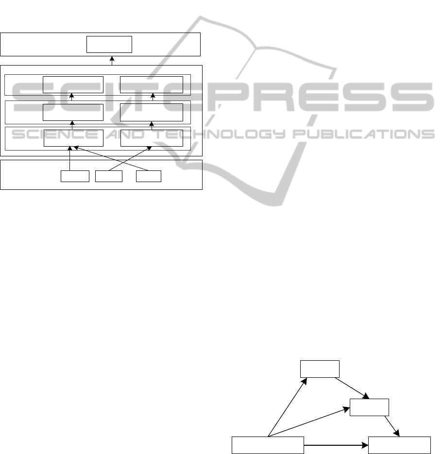
an abstraction hierarchy.

TOTAL COST

JOBS

RESOURCE 1

...

JOBS

RESOURCE

ORDER OF JOBS

RESOURCE 1

...

ORDER OF JOBS

RESOURCE R

...

JOB 1 JOB 2 JOB N

Schedule

Resources

Assignment

Sequencing

Jobs

Level1

Level2

Level3

COST RESOURCE 1

...

COST RESOURCE R

Quality

Figure 1: Abstraction levels for scheduling tasks.

The hierarchy we chose is shown in Figure 1.

From top to bottom, it reveals different levels of

detail of a general schedule. At level 1 the only

information used is the objective value of the overall

schedule. The underlying level 2 reveals details of

the sub-schedules for each resource including the

assignment of jobs to vehicles and, zooming in

further, the order of the particular jobs. The lowest

level 3 contains the individual jobs that hold their

start times and resources as properties.

A scheduling action at a certain level can be

defined without information of the underlying levels.

Consider for instance the goal of changing the

resource affiliation of a job. It is irrelevant for the

human operator where the job is positioned within

the sequence of jobs or at which time it starts.

However, for the preference to take effect a decision

about the start time has to be made in order to obtain

a schedule that does not violate any hard constraints.

That means, the level a preference targets and the

level at which it is implemented can be different. We

describe this with the term “loss of abstraction”.

3 INVESTIGATING THE HUMAN

CONTRIBUTION TO

SCHEDULING

Manual optimization of schedules is a monotonous

job unsuitable for humans (Burstein and Holsapple,

2008). Due to the structure of the problems the

number of valid positions for jobs is exponential

(Burke and Kendall, 2005) which makes it difficult

for the human to find the optimal costs. In contrast,

it is important for the user to collect and interpret the

data of schedules to find preferences and

modifications. Having identified them, he

participates in the adaptation of the schedule.

3.1 Making Decisions

The decisions about how identified preferences and

modifications are incorporated should be left to the

human in order to prevent problems of the kind we

have described in section 1.

3.1.1 Decision-making in General

Scheduling can be modeled as decision process

(Higgins, 1999) consisting of intelligence, design

and choice (Turban et al., 2010). The intelligence

phase involves the recognition of the problem at the

start of the decision process. After that, possible

solutions are evaluated in the design phase. The best

alternative is finally selected in the choice step. We

add a completion step, if the selected solution yet

has to be completed. If the completion step is still

complex, a new decision process is triggered. The

decision processes are chained that way until the

task is accomplished.

The decision process is influenced by skills and

knowledge of the human. We distinguish skill-based

(SBB), rule-based (RBB) and knowledge-based

reasoning (KBB) (Rasmussen, 1983). As shown in

Figure 2 RBB and SBB shorten the decision process.

INTELLIGENCE

DESIGN

CHOICE

SBB

COMPLETION

KBB

Figure 2: Stages in decision-making and shortcuts.

DesignofHuman-computerInterfacesinSchedulingApplications

221

Table 1: Types of reasoning.

KBB No pattern can be used. Intelligent reasoning

is required. KBB coincides with the design

phase.

RBB Familiar patterns in the data map to a rule that

implies the action.

SBB Perception is mapped to action directly.

3.1.2 Decision-making in Scheduling

The decision stages can be directly applied to human

scheduling activities.

Design: In the design stage the human operator

compares alternative solutions for the task.

Depending on the abstraction level this involves

comparing

• different schedules (level 1)

• different assignments of jobs to resources(level 2 )

• different orders of jobs within a resource (level 2)

Each considered alternative is evaluated with regard

to optimality and practicability.

However, only valid schedules can be evaluated.

Due to the earlier mentioned “loss of abstraction”

the human operator has to make decisions about the

details below the abstraction level of the task. This

leads to a new decision process in order to find a

valid implementation of the solution to be

considered. The original decision process is

compromised, as the human must keep track of

nested design stages at different levels.

Choice and Completion: The human operator

chooses the best suited schedule. If complete

schedules are compared in the design stage the

completion step can be omitted.

It depends both on the experience of the human

operator and on the characteristics of the task

whether the decision process can be shortened by

SBB or RBB.

SBB: The scheduling task is a pure optimization

of cost functions if no alternative solutions exist or if

the preference is formulated as a hard constraint.

Furthermore, typical modifications such as the

addition of jobs sometimes do not require an

evaluation in terms of practicability but only in

terms of optimality and thus are skill-based.

RBB: Applies, if the human operator deals with

the task repeatedly or if there are best practices, such

that the best suited alternative is known from

experience. The human operator has to implement

the chosen alternative in the completion step.

4 DESIGN OF INTERACTIVE

SCHEDULING INTERFACES

4.1 Hypothesis for Optimal Decision

Support

It is an important issue for decision support to keep

the human operator at the level of abstraction, that is

related to his preference and to the current type of

reasoning. For SBB and RBB the computer can

undertake the whole work of optimizing at level 1.

In KBB the scheduler should be able to test the

outcome of decisions in the design phase while

disregarding low-level constraints. To overcome the

loss of abstraction the system has to provide the

level of automation, that is needed for a particular

action.

We define the levels of automation according to

the levels of abstraction shown in Figure 2.

Level 3: This level requires the least amount of

automation, as the human operator undertakes all

decisions about start times, orders, resources and

other properties of jobs. However, to prevent faulty

decisions, the system should supervise the

compliance with the underlying constraints. In doing

so it is not sufficient to show an error message as

soon as a constraint is violated. We rather suggest to

visualize the scope of action already when the

human is about to make a decision. According to the

types of constraints in section 2.1 this means

highlighting valid properties for the considered job

that

a) meet its individual constraints

b) meet its constraints in relation to other jobs

with regard to the state of the current schedule. This

way the human does not have to make the effort to

withdraw a faulty decision.

Level 2: The human makes decisions on some

selected properties of either individual jobs or the

schedule only. The computer is required to solve the

remaining properties such that

a) all constraints are satisfied

b) the schedule is optimal or at least good with

regard to the cost function.

This is especially important for KBB, as it allows

the human operator to try and evaluate several

assignments that are based on his manual decision.

The portion of work of the computer increases with

the sublevels as shown in Table 3. At the quality

sublevel the human defines the cost function for the

scheduling of one or more jobs. In case all jobs are

chosen the decision support is equal to level 1.

ICEIS2012-14thInternationalConferenceonEnterpriseInformationSystems

222

Table 2: Properties assigned by human and computer at

different sublevels of level 2.

Sublevel Human Computer

Sequencing

resource, relative

position, cost function

start time

Assignment

resource, cost

function

relative

position, start

time

Quality cost function

resource,

relative

position, start

time

Level 1: Full automation is applied at this level. The

human operator is only concerned about the cost

function the computer should use to optimize the

whole schedule.

To sum up, the human operator decides, how

much details he contributes to a change of the

schedule.

4.2 Interactive Decision Support

Features

We have designed a set of interaction features that

can be used to build a scheduling interface providing

the recommended decision support. They are

described in Table 4. We neglect commonly used

features like Undo/Redo, as they can be found in the

standard literature about successful user interface

design (Shneidermann, 2010).

At level 3 we use colors to visualize the domain

of the property of a job in the current schedule. For

level 2 we suggest the use of controls that allow the

human operator to select a group of jobs for

optimization. This is a simple way to deal with

optimization preferences, as different objective

functions can be chosen for different groups. The

FO-feature is suited for tasks at level 1.

Fixation covers all three levels. It is the

prerequisite for all other features, as it deals with the

way the human operator enters a condition for a

certain property in the interface. Having done this

the computer considers the condition in optimizing

or constraint highlighting. Properties that are not

fixed to a certain value can be automatically

resolved with level 2 and level 1 features.

Furthermore, fixation allows keeping decisions

made at lower levels when using features at higher

levels. For example, if the human operator modifies

some jobs with the help of ECH and FIT, he can fix

their properties at level 3. If FO is applied

afterwards, the modified jobs are not changed

anymore. Figure 3 shows the abstraction levels the

features belong to.

Table 3: Decision support features.

Full Optimization

(FO)

A control to optimize the whole

schedule. It allows choosing

from various built-in cost

functions.

Single Job

Optimization (SJO)

The interface allows to select a

single job in the schedule and

triggers automatic optimization

of its position. Remaining jobs

in the schedule are kept

unchanged.

Resource

Optimization (RO)

Like SJO. All jobs belonging to

the same resource can be

selected at once.

Group Optimization

(GO)

Like SJO. Any group of jobs

from different resources can be

selected.

Fit-in (FIT)

The interface allows the user to

define the position of a job

within the sequence and looks

for a valid start time.

Constraint

Highlighting (CH)

The interface recognizes the

intention to change a property

of a job and colors possible

values

red, if they are invalid

green, if they are valid

with regard to constraints of the

individual job.

Enhanced

Constraint

Highlighting (ECH)

Additional to CH: values of

properties, that violate

constraints in relation to other

jobs are colored

yellow, if the value can be

applied as soon as the properties

of conflicting jobs are adapted

grey, if the value can never be

applied in conjunction with the

conflicting jobs.

Fixation (FIX)

The interface allows the direct

input of the desired properties

of one or more jobs. They are

turned into additional

constraints to be considered by

all features.

4.3 Example Interfaces

Our hypothesis does not include recommendations

about how to support the identification of

preferences and modifications. This is an issue for

the graphical information visualization of the

specific scheduling application. It should follow the

principles of Ecological Interface Design (Vicente,

2002), (Vicente and Rasmussen, 1992) and display

information according to the abstraction hierarchy.

We show two example interfaces that include our

recommended DSS features.

DesignofHuman-computerInterfacesinSchedulingApplications

223

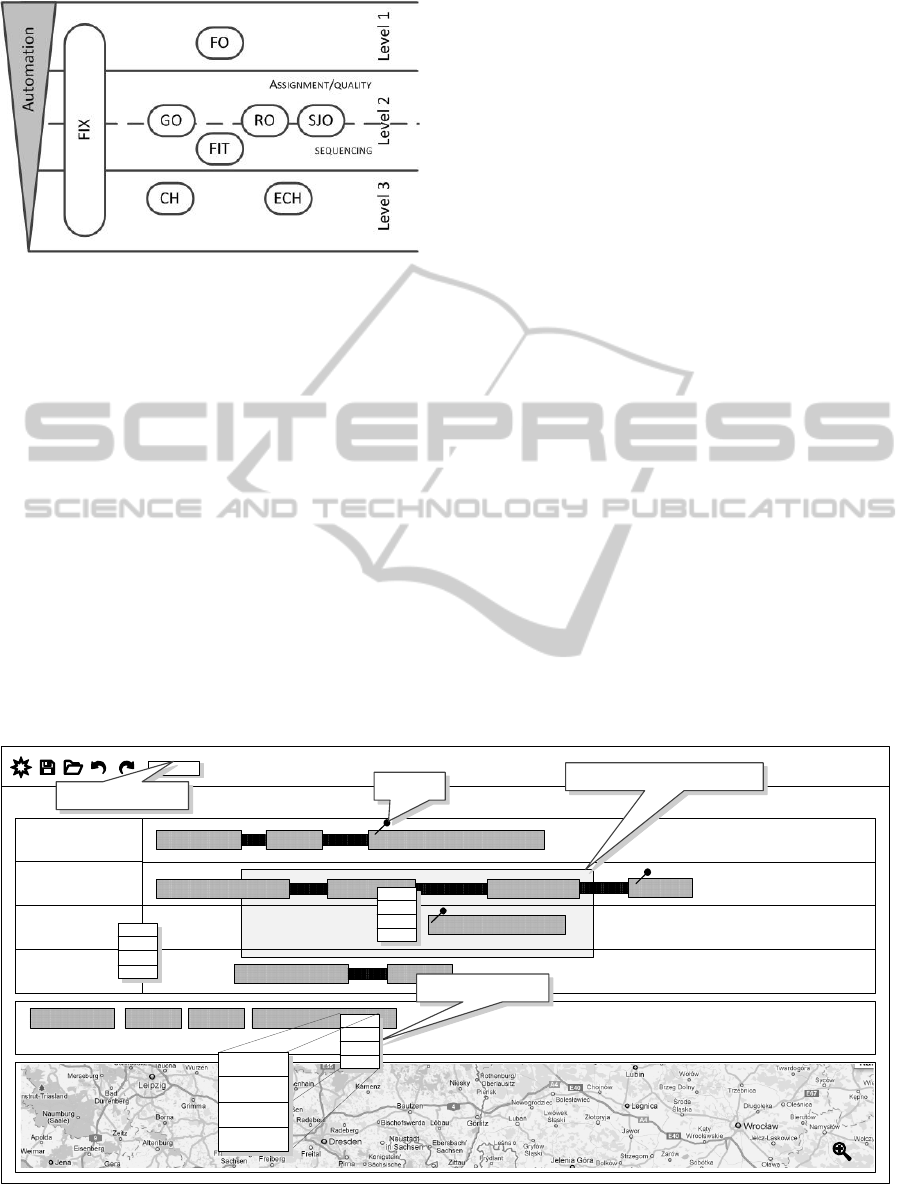
Figure 3: DSS features at different abstraction levels.

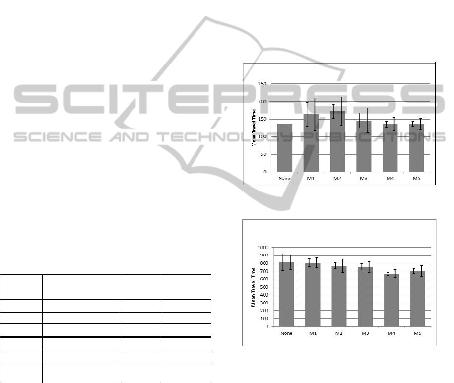
4.3.1 Fleet Scheduling

The interface used in our experiments is sketched in

Figure 4. We decided to use a Gantt chart, as it

clearly shows the sequence of jobs in time and the

travel times between them. This makes it easy to

analyze start times and resources of jobs in order to

derive certain preferences. For further support we

provide a map.

The human operator can move the jobs per Drag

and Drop. If he starts dragging constraint

highlighting is applied to the Gantt chart: the colors

of the positions show whether there are time window

conflicts or overlaps with other jobs in case the job

is dropped there. A job can be dropped at any

position colored green or yellow, in the latter case

the fit-in feature can be used to put the job correctly

in the sequence.

Furthermore SJO, RO and GO are available

through context menus and provide the two cost

functions introduced in section 2.1. Scheduling

preferences can be defined in property dialogs and

by using the pin (FIX) that fixes both start time and

resource of a job. A button to create schedules from

scratch (FO) is also provided.

4.3.2 Nurse Rostering

A possible interface for nurse rostering is shown in

Figure 5. In contrast to the vehicle routing interface

the jobs are not grouped by their resource (nurse),

but by the shift they belong to. Each shift requires a

certain number of nurses which corresponds to the

number of jobs that must be included. The cost

function usually deals with considering the

preferences of the individual nurses.

The start time of a shift determines the start

times of the associated jobs. Their resources can be

chosen from a drop-down menu, whose entries are

colored according to CH and ECH. For example, if a

nurse had a night shift the day before it must not be

assigned to the early shift due to legal requirements.

However, if the selection of this nurse is colored

yellow, the human operator is able to ask the system

to reschedule the day before such that the early shift

becomes valid. Furthermore the interface contains

features to select a group of jobs (SJO, GO) or the

whole schedule (FO) for automatic optimization. In

this case fixed nurses (FIX) are kept unchanged.

VEHICLE 1

VEHICLE 2

VEHICLE 3

VEHICLE 4

MAP

CLIPBOARD

GANTT CHART

GROUPING OF JOBS

FIXATION

CONTEXTMENUS

OPTIMIZE SCHEDULE

OPTIMIZE

FIT

‐IN

OUT

PROPERTIES

Figure 4: Interface Design for Vehicle Routing.

ICEIS2012-14thInternationalConferenceonEnterpriseInformationSystems

224

MONDAY TUESDAY WEDNESDAY

SHIFT1 SHIFT2 SHIFT3 SHIFT1 SHIFT2 SHIFT3 SHIFT1 SHIFT3SHIFT2

NURSE 1

NURSE 4

NURSE 10

URSE 12

URSE 2

NURSE 3

NURSE 5

URSE 6

...

......

URSE 2

URSE 7

URSE 8

URSE 11

NURSE 1

NURSE 2

NURSE 5

NURSE 11

DROP‐DOWN MENU

CONSTRAINT

HIGHLIGHTING

GROUP SELECTION

SCHEDULE WEEK

SCHEDULE DAY SCHEDULE DAY SCHEDULE DAY

SCHEDULE SELECTION SCHEDULE SELECTION SCHEDULE SELECTION

FULL OPTIMIZATION

GROUP OPTIMIZATION

JOBS

FIXATION

Figure 5: Interface design for Nurse Rostering.

5 EVALUATION OF THE

DECISION SUPPORT

5.1 Combining DSS Features to

Interaction Models

In order to prove our claims from section 1 it

remains to provide an empirical evaluation of

a) the suitability of the features for performing

scheduling tasks at different abstraction levels

b) the quality that can be achieved in terms of the

cost function.

For this we combine DSS features to 5

interaction models located at different abstraction

levels. They are shown in Table 5.

Model 1/2: manual scheduling at level 3

Model 3: FO at level 1, subsequent manual

modifications at level 3 are allowed, fixation is not

allowed

Model 4: like model 3, fixation is allowed

Model 5: level 2, fixation can be achieved

indirectly by excluding manually positioned jobs

from optimization groups.

Several test tasks with scheduling preferences at

different abstraction levels are carried out by peer

groups. Each model is used for each task.

5.2 Setup of the Usability Test

We have formed 5 test groups each consisting of 7

students from different faculties of our institution.

The subjects were asked to perform 6 scheduling

tasks. The models available for the particular tasks

were dependent on the test group. We determine the

best model for each task by comparing the average

performance and confidence interval in the

following metrics: accumulated travel time, task

completion, time effort, number of undo operations

and number of manual interactions. The tests took 3

hours per participant including a briefing of 30

minutes at the start. The maximum duration for each

task was set to 15 minutes.

5.2.1 Design of the Test Tasks

The participants had no experiences in scheduling.

Therefore the relevant scheduling preferences that

would otherwise arise from the expert knowledge of

the scheduler had to be predefined for each task.

1. Schedule a set of jobs such that the total travel

time is minimized and the workload

is balanced

between the resources. For some jobs there are

precedence constraints (level 2 sequencing).

2. Schedule a set of jobs such that the total travel

time is minimized and the workload is balanced.

For some jobs fixed start times and resources are

given (level 3).

3. An additional vehicle is to be utilized. Change

the given schedule such that some suitable jobs are

assigned to it (level 2 assignment).

4. An event occurs and requires an additional job.

The working schedule must include the job as

early as possible, but it has to remain unchanged

until 10 o’clock (level 3).

The workload corresponds to the total number of jobs that a

resource has to carry out.

DesignofHuman-computerInterfacesinSchedulingApplications

225

5. Schedule a set of jobs such that the total travel

time is minimized and the workload is balanced.

Jobs beyond the German-Polish border must be

carried out in one piece (level 2 sequencing).

6. Change the current schedule such that vehicle 3

finishes work at 12 o’clock. Remaining jobs have

to be assigned to other vehicles (level 2

assignment).

The tasks are to be carried out with 4 vehicles

and about 25 predefined jobs. All jobs have time

window and resource constraints. The participants

always have to strive for a compromise between low

travel time and balanced workload (level 2

quality/level 1).

5.2.2 Assignment of Test Groups to

Interaction Models

The table below shows the distribution of test

persons to different models. The models are divided

into two areas: manual optimization (model 1 and 2)

and automated optimization (models 3, 4 and 5). The

participants first carried out their tasks manually and

then repeated them with the help of automatic

features.

The assignment of models to groups changes

from task to task. This ensures that each group deals

at least one time with each interaction model. We

assigned fewer participants to models that were

expected to be very difficult (model 1 and the model

without any features) or discouraging for the test

subjects.

Table 4: Example peer groups and models for task 1.

Model Features Persons

Group

(Task 1)

- - 7 1

Model 1 CH 7 2

Model 2 ECH 21 3,4,5

Model 3 FO + ECH 7 1

Model 4 FO + FIX + ECH 14 2,3

Model 5

SJO + GO + RO +

FIX + FIT + ECH

14 4,5

5.3 Results

5.3.1 Usability Metric 1: Travel Time

In Figure 9-13 the achieved qualities of the

schedules are shown for each particular task. The

average qualities are influenced by the number of

successfully completed tasks. Both task 6 and task 1

turned out to be insoluble for our testers in 15

minutes if no decision support was provided.

Consequently, we cannot present further results.

Level 3 Tasks: The results for task 2 and 4 are

shown in Figures 6 and 7. The schedules created

with level 3-features only were worse than those

created with higher-level-features. This confirms the

assumption that skill-based scheduling tasks should

be carried out by the computer. CH and ECH help

the human to find a scheduling decision for some

jobs, but are not sufficient for creating complete

schedules.

Comparing models 3 and 4, the quality decreases

if fixation is not allowed. This suggests that

preferences should be incorporated in advance (FIX)

rather than after automated optimization.

Lefterrorinterval:confidence(90%)

Righterrorinterval:standarddeviation

Figure 6: Mean travel time – task 2.

Lefterrorinterval:confidence(90%)

Righterrorinterval:standarddeviation

Figure 7: Mean travel time – task 4 (task 5 is very similar).

Level 2 Tasks: The results for tasks 1, 3, 5 and 6 are

shown in Figures 7, 8, 9 and 10. They are similar to

those for the level 3 tasks. The best schedules mostly

result from models 4 and 5. There is no significant

difference in the performance of the two models,

which applies to all test tasks too.

The overall ranking of the models is shown in

Figure 11 (1 is the best, 6 the worst rank). It

confirms the assumption that models 4 and 5

generally provide the best decision support.

ICEIS2012-14thInternationalConferenceonEnterpriseInformationSystems

226

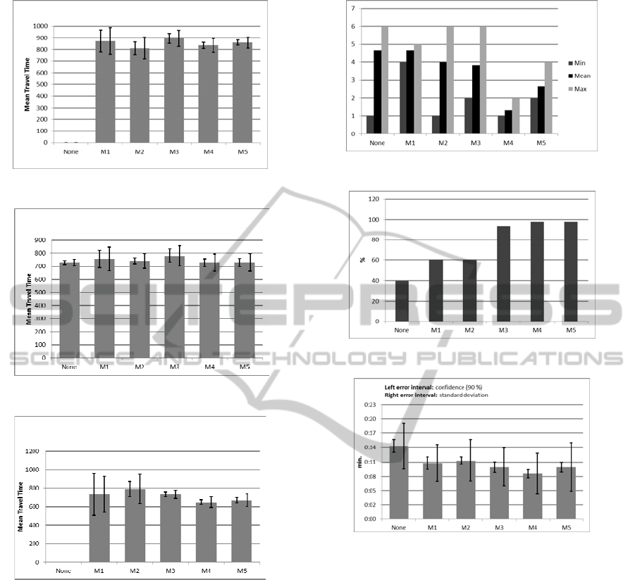
Figure 8: Mean travel time – task 1.



Lefterrorinterval:confidence(90%)

Righterrorinterval:standarddeviation

Figure 9: Mean travel time – task 3.

Left error interval: confidence

(90%) Right error interval: std.-dev.



Figure 10: Mean travel time – task 6.

5.3.2 Usability Metric 2: Task Success

The number of participants that have managed to

obtain a solution is shown in Figure 12. A task was

considered successful, if the schedule did not violate

any time window or resource constraints and the

scheduling preferences were fulfilled.

With models 1, 2 and “None” many participants

ran into dead-ends, where they were not able to

insert further jobs in the clipboard. In this case

model 2 merely depicted a grey Gantt chart

background. They would have to manually

backtrack former decisions. However, testers would

rather give up at this point.

Figure 11: Ranking of the models averaged over the tasks.

Figure 12: Rate of successful task completion.

Figure 13: Average task duration.

5.3.3 Usability Metric 3: Task Duration

The average time, users required to solve the tasks

(deadline was 15 minutes) is shown in Figure 13.

Although the time needed with no model is

particularly high, in general the models have a high

variance in their execution time. How much time a

test person spent to fulfill a task was strongly

dependent on his motivation and ideas to improve

the schedule. The runtime of the system to solve the

scheduling problem was negligible.

5.3.4 Metric 4: Interaction Frequency

Figure 14 shows the number of undo operations

averaged over the number of participants. Models 4

and 5 have a strikingly high occurrence of undo,

which refers to the general behavior in the design

phase, if there are high-level scheduling features. It

DesignofHuman-computerInterfacesinSchedulingApplications

227

consists of alternately applying and reversing

automated scheduling features until a satisficing

solution is found. Model 1 has a small peak in undo-

operations, as there is no aid to predict if an

operation will be feasible. Model 2 compensates for

this with the background-color grey.

Figure 14: Average number of undo operations.

Figure 15: Average number of manual operations.

Figure 18 shows the average number of manual

operations (drag and drop of jobs). As expected the

manual effort is the higher, the less support is

provided. However, manual scheduling is not

completely replaced by automated features, as the

user performs subsequent changes or sets certain

jobs according to his ideas.

6 CONCLUSIONS

We proposed 8 interaction features to enhance

human interaction in scheduling. These features

were evaluated in a quantitative study (usability test)

with regard to 4 relevant metrics. The results are:

1. The practicability of resulting schedules

improves with features to manually fixate, reorder

and optimize groups of jobs.

2. The success rate (solved tasks in given time) is

highly influenced by the availability of automated

scheduling features.

3. Automated scheduling features encourage the

user to explore his scope of action on the basis of

trial and error (optimize - undo).

REFERENCES

Burstein, F. and Holsapple, C. W. (Eds.). (2008).

Handbook on Decision Support Systems 1 and 2.

Springer.

Burstein, M. H. and McDermott, D. V. (1997). Issues in

the development of human-computer mixed initiative

systems. Cognitive Technology, 285-303.

Burke, E. K. and Kendall, G. (2005). Search

methodologies: introductory tutorials in optimization

and decision support techniques. Heidelberg:

Springer.

Fransoo, J. C., Waefler, T. and Wilson, J. R. (2011).

Behavioral Operations in Planning and Scheduling.

Springer.

Higgins, P. G. (1999). Job Shop Scheduling: Hybrid

Intelligent Human-Computer Paradigm. Ph.D. diss.,

Department of Mechanical and Manufacturing

Engineering, The University of Melbourne,

Melbourne, Australia.

Kallehauge, B., Larsen, J., Madsen, O. and Solomon, M.

(2005). Vehicle Routing Problem with Time

Windows. In Desaulniers, G., Desrosiers, J. and

Solomon, M. M. (Eds.), Column Generation (pp. 67-

98). Springer US.

Rasmussen, J. (1983). Skills, rules, and knowledge;

Signals, Signs and Symbols, and Other Distinctions in

Human Performance Models. IEEE Transactions on

Systems, Man, and Cybernetics, 13(3), 157-266.

St-Cyr, O. and Burns, C.M. (2001). Mental Models and

the Abstraction Hierarchy: Assessing Ecological

Compatibility. Proceedings of the Human Factors and

Ergonomics Society 45th Annual Meeting, 297-301.

Shneidermann, B. (2010). Designing the User Interface.

Pearson Addison-Wesley.

Turban, E., Sharda, R. and Delen, D. (2010). Decision

Support and Business Intelligence Systems. Prentice

Hall, Pearson.

Vicente, K. J. (2002). Ecological Interface Design:

Progress and Challenges. The Journal of the Human

Factors and Ergonomics Society, 44, 62-78.

Vicente, K. J. and Rasmussen, J. (1992). Ecological

interface design: theoretical foundations. IEEE

Transactions on Systems, Man, and Cybernetics,

22(4), 589-606.

Wezel, W., Jorna, R. and Meystel, A. (Eds.). (2006).

Planning in Intelligent Systems.Wiley Interscience.

ICEIS2012-14thInternationalConferenceonEnterpriseInformationSystems

228