On Continuous Top-k Similarity Joins

Da Jun Li

, En Tzu Wang

, Yu-Chou Tsai

and Arbee L. P. Chen

Department of Computer Science, National Tsing Hua University, Hsinchu, Taiwan, R.O.C.

Cloud Computing Center for Mobile Applications, Industrial Technology Research Institute, Hsinchu, Taiwan, R.O.C.

Institute for Information Industry, Taipei, Taiwan, R.O.C.

Department of Computer Science, National Chengchi University, Taipei, Taiwan, R.O.C.

Keywords: Data Stream, Similarity Join, Continuous Query, Top-K Query.

Abstract: Given a similarity function and a threshold

within a range of [0, 1], a similarity join query between two

sets of records returns pairs of records from the two sets, which have similarity values exceeding or

equaling

. Similarity joins have received much research attention since it is a fundamental operation used

in a wide range of applications such as duplicate detection, data integration, and pattern recognition.

Recently, a variant of similarity joins is proposed to avoid the need to set the threshold

, i.e. top-k

similarity joins. Since data in many applications are generated as a form of continuous data streams, in this

paper, we make the first attempt to solve the problem of top-k similarity joins considering a dynamic

environment involving a data stream, named continuous top-k similarity joins. Given a set of records as the

query, we continuously output the top-k pairs of records, ranked by their similarity values, for the query and

the most recent data, i.e. the data contained in the sliding window of a monitored data stream. Two

algorithms are proposed to solve this problem. The first one extends an existing approach for static datasets

to find the top-k pairs regarding the query and the newly arrived data and then keep the obtained pairs in a

candidate result set. As a result, the top-k pairs can be found from the candidate result set. In the other

algorithm, the records in the query are preprocessed to be indexed using a novel data structure. By this

structure, the data in the monitored stream can be compared with all records in the query at one time,

substantially reducing the processing time of finding the top-k results. A series of experiments are performed

to evaluate the two proposed algorithms and the experiment results demonstrate that the algorithm with

preprocessing outperforms the other algorithm extended from an existing approach for a static environment.

1 INTRODUCTION

Given a similarity function and a threshold

within

a range of [0, 1], a similarity join query between two

sets of records returns pairs of records from the two

sets, which have similarity values equal to or higher

than

. The similarity join query has received

considerable attention since it is a fundamental

operation in a wide range of applications such as

page detection (Henzinger, 2006), data integration

(Cohen, 1998), data de-duplication (Sarawagi and

Bhamidipaty, 2002), and data mining (Bayardo et al.,

2007). The literatures on similarity joins can be

roughly categorized into two types, one for

computing approximate similarity values (Broder et

al., 1997) (Chowdhury et al., 2002); (Charikar, 2002)

(Gionis et al., 1999) and the other for computing

exact similarity values (Chaudhuri et al., 2006)

(Bayardo et al., 2007) (Sarawagi and Kirpal, 2004);

(Xiao et al., 2008).

In (Broder et al., 1997), documents are divided

into several continuous subsets and then, these

subsets are employed to approximately identify the

near duplicate web pages. Local Sensitive Hashing

(LSH) (Gionis et al., 1999) is a widely adopted

technique for solving the approximate similarity join

problem. The basic idea of LSH is to hash the data

from the databases to ensure that the probability of

collision is much higher for objects that are close to

each other than for those that are far apart. Several

approaches use LSH to obtain the guarantees of the

probability of false positive and that of false

negative. (Gionis et al., 1999) applies LSH to detect

the duplicates of data with high dimensions.

(Chowdhury et al., 2002) uses the collected statistics

to detect the duplicate documents. (Charikar, 2002)

proposes a new LSH scheme to estimate similarity

Jun Li D., Tzu Wang E., Tsai Y. and L. P. Chen A..

On Continuous Top-k Similarity Joins.

DOI: 10.5220/0003993200870096

In Proceedings of the International Conference on Data Technologies and Applications (DATA-2012), pages 87-96

ISBN: 978-989-8565-18-1

 2012 SCITEPRESS (Science and Technology Publications, Lda.)



and based on that, a randomized algorithm is also

proposed. The other type of literatures on similarity

joins returns the exact answers. Based on various

index techniques and filtering principles, several

approaches such as (Sarawagi and Kirpal, 2004);

(Chaudhuri et al., 2006) (Bayardo et al., 2007);

(Xiao et al., 2008) have been proposed. (Bayardo et

al., 2007) proposes a principle to quickly access

inverted lists. (Xiao et al., 2008) designs a novel

technique to index and process the similarity join

queries. (Arasu et al., 2006) divides the records into

partitions and hashes them into signatures. It also

employs a post filtering step to prune the pairs of

records for reducing candidates.

As mentioned, the original similarity join needs a

user-given threshold, yet setting a suitable threshold

may not be easy without the background knowledge

to the given datasets. Therefore, Xiao et al. propose

a variant of similarity joins, i.e. the top-k similarity

join query in (Xiao et al., 2009), which returns the k

pairs of records from the given two sets of records,

with the highest similarity values. In (Xiao et al.,

2009), the topk-join approach, to be formally

introduced in the next section, is proposed to deal

with the top-k similarity join query. Its main idea is

to quickly compute the upper bounds of similarity

values related to pairs of records and then prune the

candidate results if their upper bounds are lower

than the similarity value of the temporal k

pair of

records. Consider a scenario as follows. A blogger

writes some articles in her/his blog and is interested

in the other blog articles highly related to these

articles. As blog articles are continuously generated,

able to be regarded as an article data stream, the

above scenario can be turned into the problem of

continuous top-k similarity joins. Since users often

concern more about the recent data, we adopt the

sliding window model in this paper. Given a set of

records being regarded as a query and a sliding

window over a data stream, the continuous top-k

similarity join query returns k pairs of records

regarding the query and the data contained in the

sliding window, which have the highest similarity

values.

To deal with this problem, we can apply the

topk-join approach (Xiao et al., 2009) whenever the

window slides. Obviously, we can improve this

solution since most of the data in the current window

are identical to those in the last window. We first

propose a solution extended from the topk-join

approach, which computes the top-k results

regarding the query and newly arrived data as

candidate results and derives the join results from

the candidate set. Moreover, we propose another

algorithm preprocessing the query in advance,

making the data able to be compared with all the

records in the query at one time. Our contributions

can be summarized as follows. 1) We make the first

attempt to address the problem on continuous Top-k

similarity joins in this paper. 2) We also propose two

algorithms for solving this problem, one extended

from the topk-join approach proposed in (Xiao et al.,

2009) and the other one based on preprocessing the

issued query for parallel comparisons of the records.

The rest of the paper is organized as follows. The

preliminaries are introduced in Section 2, including

the problem formulation and the topk-join approach

(Xiao et al., 2009). Thereafter, the proposed

solutions are detailed in Section 3. The experiment

results are presented and analyzed in Section 4 and

finally, Section 5 concludes this work.

2 PRELIMINARIES

To deal with the traditional problem of similarity

joins, a user needs to set a similarity threshold to

identify which join results s/he is interested in. In

(Xiao et al., 2009), Xiao et al. turn to solve a variant

of the similarity join problem, i.e. top-k similarity

joins. Without the need to set the threshold, in the

top-k similarity join problem, the join results with

the k highest similarity values are returned. Next, the

problem of top-k similarity joins and the

corresponding solution proposed in (Xiao et al.,

2009) are introduced in Subsection 2.1, followed by

the problem of continuous top-k similarity joins,

formulated in Subsection 2.2.

2.1 Introduction to Top-k Similarity

Joins

Let I = {W

, W

, …, W

|I|

} be a finite set of symbols

(literals) called tokens. A record is considered as a

set of tokens. Given a similarity function denoted

sim(⋅, ⋅), which returns a similarity value s ∈ [0, 1]

between two records, top-k similarity joins between

two sets of records return k pairs of records that have

the highest similarity values. Notice that, we focus

on Jaccard similarity function in this paper;

accordingly, sim(x, y) is equal to

||||

yxy∩∪

where x and y are records.

A solution to the problem of top-k similarity

joins, proposed in (Xiao et al., 2009), is mainly

based on the concept of prefix filtering (Chaudhuri

et al., 2006); (Xiao et al., 2009) described as follows.

Suppose that the tokens of two records x and y are

DATA2012-InternationalConferenceonDataTechnologiesandApplications



each sorted into a common order, e.g. an alphabet

order, and the p-prefix of a record x is defined as the

first p tokens of x. If sim(x, y) ≥ α, then

the

()

|| || 1xx

−+

⎡⎤

⎢⎥

-prefix of x and

the

(

)

|| || 1yy

−+

⎡⎤

⎢⎥

-prefix of y must share at least

one token, where α ∈ [0, 1] and |x| is the cardinality

of x. For example, let α, the sorted x, and the sorted y

be 0.5, {A, C, E, G, J}, and {D, E, G, J},

respectively. Since sim(x, y) = 0.5 = α, the 3-prefix

of x, i.e. {A, C, E}, and the 3-prefix of y, i.e. {D, E,

G}, share at least one token, say E. In other words, if

the

(

)

|| || 1xx

−+

⎡⎤

⎢⎥

-prefix of x and

the

(

)

|| || 1yy

−+

⎡⎤

⎢⎥

-prefix of y do not share any

common tokens, sim(x, y) must be smaller than α,

which is the main pruning rule used in the topk-join

algorithm proposed in (Xiao et al., 2009).

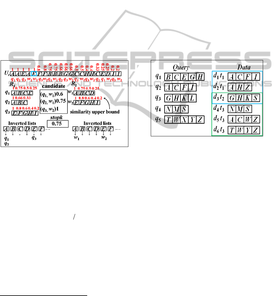
Figure 1: Similarity upper bounds and inverted lists used

in the topk-join algorithm.

Given two sets of records R

and R

, each record

in either R

or R

is assumed to be sorted into a

common order as described in (Xiao et al., 2009)

Then, each token in a record is associated with a

pre-computed similarity upper bound. The similarity

upper bound of the token in the p

position of a

record x is equal to

(

)

1( 1)||px−−

. For example, as

shown in Figure 1, each token of the record q

, i.e. A,

B, C, and E, has a corresponding similarity upper

bound, i.e. 1, 0.75, 0.5, and 0.25. The similarity

upper bound of the token in the p

position of x

means if any record, say y, satisfies that y and the (p

− 1)-prefix of x do not share any one token, sim(x, y)

must be smaller than or equal to the corresponding

similarity upper bound. The topk-join algorithm

(Xiao et al., 2009) works as follows. Let U

be a



In [XW09], tokens in each record are sorted into an increasing

order of occurrence frequency for efficiency.

multi-set of tokens, consisting of all tokens of all

records in the two sets R

and R

. Moreover, R

and

are each associated with a set of inverted lists as

shown in Figure 1. Each token in U

is processed in a

decreasing order of the similarity upper bound. As

the current processed token T is with a similarity

upper bound equal to s

, the corresponding record

of T with s

, say q contained in R

, is inserted into

the inverted list of T, regarding R

. Then, the

similarity values between q and the records

contained in the inverted list of T, regarding R

are

computed. The k highest similarity value among the

computed join results is used to be a threshold

named stopk. The more tokens contained in U

are

processed, the larger the value of stopk becomes.

Finally, the whole process stops once each

unprocessed token in U

has a similarity upper bound

smaller than stopk.

Figure 2: Continuous Top-2 similarity joins regarding a

sliding window with a size of 3.

2.2 Problem Formulation

Different from the original top-k similarity joins

considering the static sets of records, in this paper,

we make the first attempt to deal with the problem

of top-k similarity joins in a dynamic environment

involving a data stream. A data stream in this paper

is defined as an unbounded sequence of records.

Notice that, in each time slot t

, i = 1, 2, 3, …, a

non-fixed number of records may be generated in

the data stream. Since users may often be interested

in recent data, we take into account the sliding

window model, which only concerns the data

records arriving at the most recent m time slots.

More specifically, we only concern the data records

of the target stream that arrive in the time slots

between t

c−m+1

and t

, where t

is the current time slot.

Since top-k similarity joins involve two sets of

records, in addition to the data records coming from

the target stream, the other finite set of records are

issued by a user, being regarded as a continuous

OnContinuousTop-kSimilarityJoins



query. This type of records is called query records.

Then, the problem to be solved in this paper is

defined as follows. Given a set of query records and

a sliding window with a size of m, we issue a query

of continuous top-k similarity joins that continuously

returns k pairs of records with the highest similarity

values, regarding the query records and the data

records contained in the current window.

Example 1: Let both of m and k be 2. Moreover, as

shown in Figure 2, the continuous query consists of

five query records. When the sliding window

contains the time slots t

and t

, the join results are

, d

) and (q

, d

). After the window slides to

contain the time slots t

and t

, the join results

become (q

, d

) and (q

, d

3 CONTINUOUS TOP-K

SIMILARITY JOINS

A naïve solution to the query of continuous top-k

similarity joins is to repeatedly perform topk-join

(Xiao et al., 2009) for the current window whenever

the window slides. However, since most of the data

records contained in the current window are likely

identical to those contained in the last window,

performing topk-join twice may cause redundant

computation, thus inefficient. Next, we propose two

algorithms to solve the query of continuous top-k

similarity joins, focusing on computation sharing to

reduce the redundant computation.

3.1 The AllTopk Algorithm

A straightforward idea of reducing the redundant

computation mentioned above is that we keep the

top-k pairs of records regarding the current window

and once the window slides, we hope to generate

some join results only from the data records arriving

at the new time slot to obtain the top-k pairs

regarding the new window. However, the problem is

that: are the join results generated from the data

records arriving at the new time slot indeed

contained in the answer set regarding the new

window? Obviously, the answer is “no.” Even that,

this idea can be practical if we keep more candidate

join results rather than keeping only the exact top-k

pairs of records regarding the current window. The

following Lemma claims how many candidate join

results needing to be kept, deriving our first

algorithm named AllTopk.

Lemma 1: Suppose that for each new time slot t, n

pairs of records with the highest similarity values,

regarding the query records and the data records

arriving at t, are kept in a candidate result set.

Moreover, the pairs of records, associated with the

expiring time slot, are deleted from the candidate

result set whenever the window slides. Then, if n ≥ k,

the exact top-k join results regarding the current

window must be contained in the candidate result

set.

Proof: Assume that a pair of records, say (q, d) is

one of the exact top-k join results regarding the

current window yet not kept in the candidate set,

where q is a query record and d is a data record

arriving at the time slot t contained in the current

window. Since for each new time slot, n pairs of

records with the highest similarity values, regarding

the query records and the data records arriving at the

time slot are kept in the candidate set and n ≥ k, we

can infer that at least k pairs of records regarding the

data records arriving at t have the similarity values

larger than that of (q, d). Here, a contradiction

occurs. Accordingly, if n ≥ k, the exact top-k join

results regarding the current window must be

contained in the candidate set.

By Lemma 1, we propose the AllTopk algorithm that

works as follows. For each now time slot t, topk-join

(Xiao et al., 2009) is applied to find the top-k join

results regarding the query records and the data

records arriving at t and the results are kept in a

candidate set. Moreover, once a time slot expires due

to window sliding, the join results associated with

the expiring time slot are deleted from the candidate

set. By the above steps, the top-k join results

regarding the current window are always kept in the

candidate set and can be easily obtained. In Alltopk,

keeping k pairs of records with the highest similarity

values, regarding the query records and the data

records arriving at the new time slot, is needed since

keeping only n pairs of records, where n < k may

have a risk of generating the incorrect results. An

illustration below is used to describe this condition.

Example 2: As shown in Figure2, let both of m and

k be 2. If we only find the top-1 pair of records

between the query records and the data records

arriving at the new time slot, the candidate set

related to the window containing t

and t

is {(q

, d

)}, which is exactly equal to the corresponding

answer set. After the window slides to contain t

and

, (q

, d

) is deleted and (q

, d

) is inserted in the

candidate set, making the candidate set equal to {(q

), (q

, d

)}. Actually, the exact answer set

mentioned above is equal to {(q

, d

), (q

, d

)} rather

than {(q

, d

), (q

, d

)}.

DATA2012-InternationalConferenceonDataTechnologiesandApplications



3.2 The Progressive Parallel

Comparison (PPP) Algorithm

Once the continuous query, say a set of query

records, is registered, we continuously return k pairs

of records with the highest similarity values,

regarding the query records and the data records

contained in the current window. Since the query

records are fixed and need to continuously compare

with the newly generated data records, the process

will be more efficient by parallel comparing a data

record with all query records at one time. Actually,

this is the main idea of our second solution to the

problem of continuous top-k similarity joins, named

PPP (standing for Progressive Parallel comParison).

In the following, we first introduce the data structure

to be used, followed by the pruning strategy, and

then detail the PPP algorithm.

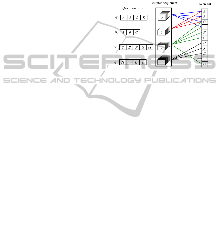
3.2.1 Data Structure

As mentioned, since the query records are fixed once

registered, we design a data structure consisting of

counter sequences and a token list to keep the

information of the query records. An example of the

data structure is shown in Figure3. Each query

record is associated with a sequence of counters,

denoted a counter sequence, which has a dynamic

size equal to the number of data records contained in

the current window. Initially, all of the counters are

set to zero. The k

counter in the counter sequence

associated with a query record q is used to count the

number of common tokens between q and the k

data record in the current window. On the other hand,

the token list is a list keeping the tokens of the union

of the query records. The tokens kept in the token

list are sorted into an alphabet order. Each token in

the token list points to the counter sequences whose

corresponding query records contain the token. For

example, token A shown in Figure3 points to the

first and second counter sequences since A is

contained in both of q

and q

The links kept in the token list help to quickly

figure out which query records contain a certain

token, and through the counters in the counter

sequences, we can easily get the number of common

tokens between a query record and a data record and

then further obtain the corresponding similarity

value. We assume that each data record is sorted into

an alphabet order. While the window slides and

some newly generated data records arrive, each of

them is processed as follows. We scan the tokens of

a data record and update the corresponding counters

in the counter sequences. More specifically, if the

current token being processed in a data record is

token A, the counters regarding the data record,

linked by token A in the token list, are all increased

by one. Once each token in a data record is

processed, we can compute the similarity values of

all pair of records regarding the data record by using

the counters related to the data record.

Figure 3: A data structure to keep the information of query

records.

3.2.2 Pruning Strategy

As mentioned in Subsection 2.1, the concept of

prefix filtering is used to solve the problem of top-k

similarity joins (Xiao et al., 2009). In the PPP

algorithm, our pruning strategy is also based on the

extension concept of prefix filtering, called extended

prefix filtering.

Lemma 2 (Extended Prefix Filtering): Suppose

that the tokens of two records x and y are each sorted

into a common order. If sim(x, y) ≥ α, then the

(

)

|| || 1 -prefixxxm

−++

⎡⎤

⎢⎥

of x and the

(

)

|| || 1 -prefixyym

−++

⎡⎤

⎢⎥

of y must share at least

(1 + m) tokens, where α ∈ [0, 1] and

{0}mZ

∈∪.■

Proof: Assume that the

(

)

|| || 1 -prefixxxm

−++

⎡⎤

⎢⎥

of x and the

(

)

|| || 1 -prefixyym

−++

⎡⎤

⎢⎥

of y share n tokens,

where n < (1 + m). In the following, it is separated

into two cases for discussion, including y < a|x| and

y ≥ a|x|.

Case 1 (y < a|x|):

sim(x, y) =

Min(||,||) ||

Max(| |,| |) | |

xy xy x

∩

∪

Case 2 (y ≥ a|x|):

Let d be the number of common tokens between the

remainder part of x and that of y. Obviously, d

OnContinuousTop-kSimilarityJoins



≤

(

)

|| || || 1

xxm

−− ++

⎡⎤

⎢⎥

()

sim(x, y)

|||| ||||

||(|| || 1+ )

|||| ||(|| || 1+ )

|| ||

|||| || 1|| || || 1

nd md

ynd x ymd

mx x x m

xymx x x m

xy x x x x

αα

ααα

∩

∪

−−

⎡⎤

⎢⎥

⎡⎤

⎢⎥

⎡⎤ ⎡⎤

⎢⎥ ⎢⎥

⎡⎤ ⎡⎤

⎢⎥ ⎢⎥

≤

+−− +−−

+− − +

≤

+−−+ − +

=≤

+− + + − +

We conclude that if n < (1 + m), then sim(x, y) < α,

which means if sim(x, y) ≥ α, then n ≥ (1 + m).

Accordingly, we demonstrate that If sim(x, y) ≥ α,

then the

()

|| || 1 -prefixxxm

−++

⎡⎤

⎢⎥

of x and

the

()

|| || 1 -prefixyym

−++

⎡⎤

⎢⎥

of y must share at

least (1 + m) tokens, where α ∈ [0, 1]

and

{0}mZ

∈∪.

3.2.3 The PPP Algorithm

In the following discussion, we assume that all of

the data records are sorted into an alphabet order

while being generated. Conceptually, the PPP

algorithm works as follows. When a new data record

arrives at the current time slot due to window sliding,

the tokens of the data record will be sequentially

processed. Notice that, as mentioned above, for each

query record, there is a counter in its corresponding

counter sequence, which is related to a certain data

record contained in the current window. If the token

being processed is T, the query records containing T

can be easily found by the link of the token T in the

token list. Then, the corresponding counters of the

linked counter sequences are increased by one. After

finishing the scanning process of a data record, we

can easily compute all of the similarity values of the

pairs of records regarding the data record by the

counter sequences. These pairs of records with

known similarity values are kept as candidate results

and then, the top-k pairs of records can be always

found from them. This is the basic idea of PPP and

actually, we can apply the extended prefix filtering

to speed up the algorithm. During the process of

scanning the tokens of a data record, once we find

that all of the join results regarding this data record

have no chances at all to be the Top-k pairs of

records in the current window, we stop processing

the remainder tokens of the data record. However,

when the window slides, since the non-Top-k pairs

of records may become the Top-k pairs of records,

we need to resume the stopped scanning process of

the data records to get their corresponding similarity

values. In the following, when to stop the scanning

process of a data record and how to resume the

stopped scanning process of a data record are

detailed.

Let α be a threshold within a range of [0, 1].

According to the prefix filtering principle, if

the

(

)

|| || 1-prefixdd

−+

⎡⎤

⎢⎥

of a data record d and a

query record q do not share any common tokens,

then processing the remainder tokens from the

position of

(

)

|| || 1 1dd

−

⎡⎤

⎢⎥

in d is not necessary

since sim(d, q) must be smaller than

. The number

(

)

|| || 1 1dd

−

⎡⎤

⎢⎥

for the data record d is

denoted ISP (standing for Initial Stop Position),

which means once we find that no tokens are shared

between the

(

)

|| || 1-prefixdd

−+

⎡⎤

⎢⎥

of d and q, sim(d,

q) must be smaller than

, thus stopping the

scanning process of d at the position

(

)

|| || 1 1dd

−

⎡⎤

⎢⎥

. Moreover, we define another

variable, i.e. SP (standing for Stop Position). Initially,

SP of d is set equally to ISP of d,

i.e.

(

)

|| || 1 1.dd

−

⎡⎤

⎢⎥

Following the extended

prefix filtering principle, if the

(

)

|| || 1 -prefixdd m

−++

⎡⎤

⎢⎥

of d and q do not share at

least (m + 1) common tokens, sim(d, q) must be

smaller than α. Accordingly, while scanning the

tokens in d, if q and d have a common token, SP of d

will be accumulated; this scanning process will stop

until the current token to be processed is at the

position of SP of d.

Algorithm 1: The PPP Algorithm

Input: W is a set of records contained in the current window.

Output: the top-k pairs of records regarding the query records and the

data records contained in W.

Variable: stopk, ISP(d), P(d), SP(d), and MI(d).

1. For each record d

∈ W

2. ISP(d) =

(

)

|| || 1 1d stopk d

−

⎡⎤

⎢⎥

3. If d is at the new time slot

4. P(d) = 1, MI(d) = 0, and SP(d) = ISP(d)

5. Else

6. Load the corresponding P and MI of d

7. For each un-scanned token t in d

8. SP(d) = ISP(d) + MI(d)

9. If P(d) ≥SP(d)

10. Store P(d) and MI(d)

11. Jump to Line 1

12. Else if t is contained in the token list

13. Accumulate the counters of the counter sequences

linked by t

14. Update MI(d) using the corresponding counters

15. Compute all similarity values of pairs of records regarding d

16. Insert these pairs of records regarding d to the candidate set and

generate the new stopk

17. Return the top-k pairs of records from the

candidate set

18. After the window slides, generate the new stopk from the

candidate set

We use an example of a query record q to specify

DATA2012-InternationalConferenceonDataTechnologiesandApplications



how to apply the extended prefix filtering principle

to the PPP algorithm as above. In fact, since the

main idea of PPP is to compare a data record with all

of the query records at one time, a variable denoted

MI (standing for Maximum Intersection), is used to

keep the largest number of the intersection between

each query record and the scanned prefix of a data

record d. Then, SP of d is always set to ISP of d plus

MI of d during the scanning process of d. MI of d

can be found from the counter sequences. Notice

that, if SP of d is larger than |d|, we need to process

each token of d and then compute the similarity

values of the pairs of records regarding d. On the

other hand, to resume the stopped scanning process

of a data record is very easy; we only need to keep

the position of the token to be processed of a data

record and its corresponding MI. After resuming the

scanning process, we continuously scan the tokens

of a data record d from the position where it stopped;

this position is denoted P of d.

Now, the whole process of PPP is detailed as

follows. Whenever the window slides, each data

record contained in the current window is

sequentially processed. If a data record d is new in

the current window, P of d, i.e. P(d), and MI of d,

denoted MI(d), are initialized, set to 1 and 0,

respectively. Moreover, ISP of d, denoted ISP

(d), is

set to

(

)

|| || 1 1d stopk d−++

⎡⎤

⎢⎥

, where stopk (playing

the same role as

discussed above) is a threshold

within a range of [0, 1], equal to the similarity value

of the pair of records which is with the k

largest

similarity value in the candidate set.

If d is not new

in the current window, its status including P(d) and

MI(d) will be restored. Then, we start to scan the

un-scanned tokens in d and also update P(d)

according to the position of the current token to be

processed. If the token being scanned in d is t, the

corresponding counters in the counter sequences

linked by t in the token list are increased by one.

Moreover, MI(d) is also updated to the largest value

of the corresponding counters. During the scanning

process, SP(d) is always set to ISP(d) plus MI(d). If

P(d) ≥

 SP(d), then all pairs of records regarding d

must have similarity values smaller than stopk, thus

able to be pruned. However, P(d) and MI(d) are kept

since the pairs of records regarding d may have

chances becoming the Top-k results in the future due

to window sliding. Once all tokens in a data record d

have been scanned, the corresponding similarity

values are computed and the pairs of records

regarding d are kept in the candidate set. In this



In the very beginning, stopk is equal to 0 since there are no

candidate results kept in the candidate set.

moment, the new stopk is reassigned using the new

candidate set. To find the answer set, we only need

to check the pairs of records kept in the candidate set.

The pseudo codes of PPP are shown in Algorithm 1.

Token list

Counter sequences

A B C

A F I J K

C E F

Candidate set

(

, 0.75)

(

, 0.6)

stopk: 0.6

SP(

): 9

ISP(

): 6

MI(

): 3

G M

W (data records)

Length of

query records

stopk: 0

(

, 0.125)

(

, 0)

Token list

Counter sequences

A B C

A F I J K

C E F

Candidate set

(

, 0.75)

(

, 0.6)

stopk: 0.6

SP(

): 9

ISP(

): 6

MI(

): 3

G M

W (data records)

Length of

query records

stopk: 0

(

, 0.125)

(

, 0)



Figure 4(1): After processing

Token list

Counter sequences

A B C

A F I J K

C E F

Candidate set

stopk: 0.6

SP(

): 5

ISP(

): 4

MI(

): 1

G M

W (data records)

Length of

query records

stopk: 0.6

(

, 0.75)

(

, 0.6)

(

, 0.125)

(

, 0)

): 5

Token list

Counter sequences

A B C

A F I J K

C E F

Candidate set

stopk: 0.6

SP(

): 5

ISP(

): 4

MI(

): 1

G M

W (data records)

Length of

query records

stopk: 0.6

(

, 0.75)

(

, 0.6)

(

, 0.125)

(

, 0)

): 5



Figure 4(2): Porcessing

and then stopping at the

position of 5.

Token list

Counter sequences

A B C

A F I J K

C E F

Candidate set

stopk: 0.75

SP(

): 9

ISP(

): 4

MI(

): 5

G M

W (data records)

Length of

query records

stopk: 0.6

(

, 1)

(

, 0.75)

(

, 0.29)

(

, 0.14)

(

, 0)

(

, 0.6)

(

, 0.125)

(

, 0)

Top-2

(

, 1)

(

, 0.75)

): 5

Token list

Counter sequences

A B C

A F I J K

C E F

Candidate set

stopk: 0.75

SP(

): 9

ISP(

): 4

MI(

): 5

G M

W (data records)

Length of

query records

stopk: 0.6

(

, 1)

(

, 0.75)

(

, 0.29)

(

, 0.14)

(

, 0)

(

, 0.6)

(

, 0.125)

(

, 0)

(

, 1)

(

, 0.75)

(

, 0.29)

(

, 0.14)

(

, 0)

(

, 0.6)

(

, 0.125)

(

, 0)

Top-2

(

, 1)

(

, 0.75)

): 5



Figure 4(3): After processing

Token list

Counter sequences

A F I J K

C E F

Candidate set

stopk: 0.29

SP(

): 7

ISP(

): 5

MI(

): 2

G M

W (data records)

Length of

query records

stopk: 0.29

A B C D H

(

, 1)

(

, 0.29)

(

, 0.14)

(

, 0)

(

, 0.125)

(

, 0.14)

(

, 0.11)

(

, 0.29)

Token list

Counter sequences

A F I J K

C E F

Candidate set

stopk: 0.29

SP(

): 7

ISP(

): 5

MI(

): 2

G M

W (data records)

Length of

query records

stopk: 0.29

A B C D H

(

, 1)

(

, 0.29)

(

, 0.14)

(

, 0)

(

, 0.125)

(

, 0.14)

(

, 0.11)

(

, 0.29)

(

, 1)

(

, 0.29)

(

, 0.14)

(

, 0)

(

, 0.125)

(

, 0.14)

(

, 0.11)

(

, 0.29)



Figure 4(4): The window slides to contain

, and

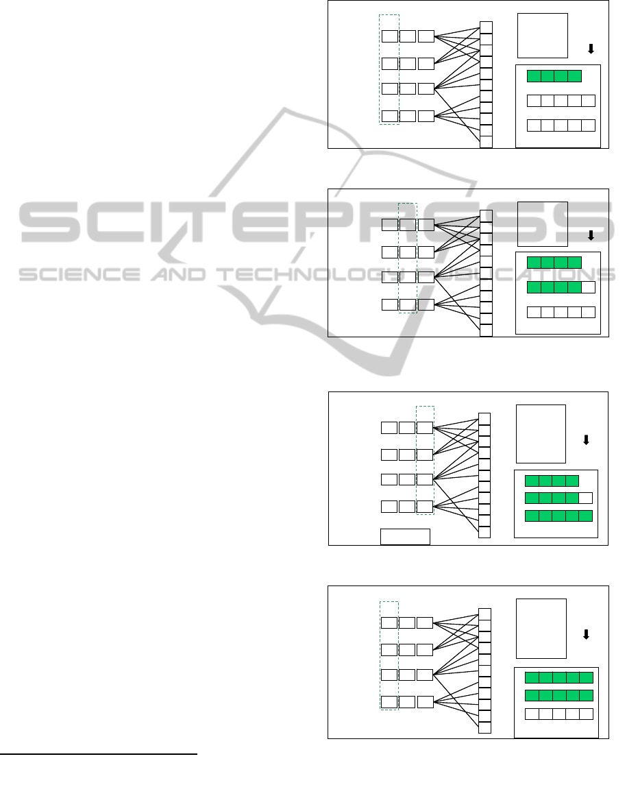
Figure 4: A running example of the PPP algorithm.

OnContinuousTop-kSimilarityJoins



Example 3:

Let k be 2. The continuous query

consists of four query records including

and

with a length equal to 4, 3, 5, and 4,

respectively. Initially, stopk is set to 0. After

processing

, stopk becomes 0.6. The candidate set

and the corresponding values of

are as shown in

Figure 4(1). In Figure 4(2), since SP(

) is equal to 5,

the scanning process stops at the position of K in

) is set to 5 for resuming the scanning process of

in the future. Then, we continue to process

shown in Figure 4(3). After processing

, stopk

becomes 0.75. Since all data records contained in W

are went through, the Top-2 pairs of records are

found from the candidate set. That is, (

, 1) and

(

, 0.75). When the window slides to contain

, and

, stopk first becomes 0.29 since

is out

of the window. Then we resume the scanning

process of

from the position of P(

4 PERFORMANCE EVALUATION

A series of experiments are performed to compare

the AllTopk algorithm and the PPP algorithm. The

experiment setup is described in Subsection 4.1 and

the experiment results are shown and analyzed in

Subsection 4.2.

4.1 Experiment Setup

In addition to comparing AllTopk and PPP, a naïve

algorithm is used to be the basis in the experiments.

How the naïve algorithm works is described as

follows. To the best of our knowledge, since the

topk-join algorithm (Xiao et al., 2009) is the

state-of-the-art solution in the static environment,

whenever the window slides, we apply topk-join to

find the results regarding the query records and the

data records contained in the current window. Naïve,

AllTopk, and PPP are all implemented in C++ and

compiled using GCC 4.1.2. Moreover, all

experiments are performed on a PC with the Intel

Core2 Quad 2.4 GHz CPU and 2GB memory.

Following (Xiao et al., 2009), we use DBLP data

from the DBLP web site to be the test dataset. We

cache the titles of papers from DBLP and treat a

paper title as a record. Moreover, paper titles are

divided into 2-grams and a 2-gram string is regarded

as a token. The total number of data records kept in

the dataset is 81790. Notice that, the order

mentioned in the algorithms follows the alphabet

order and the priority of uppercase is higher than

that of lowercase.

Table 1: The parameters used in the experiments.

Parameter Default

value

Range

Query Size 150 50~450

k 100 1~100

Window Size 2 1~8

Sliding Size 1 1~8

Time Slot Size [480, 620] [120, 140] and [480, 620]

All of the experiment parameters are shown in

Table 1 and detailed as follows. Query Size means

the number of query records. k means the number of

results to be reported. Window Size means the

number of time slots contained in the sliding

window. Sliding Size means the number of time slots

in each slide. For example, if Sliding size is 2, two

time slots are newly contained and another two time

slots expire whenever the window slides. Moreover,

to simulate an inconsistent number of data records

arriving at a time slot, the number of data records at

a time slot is randomly chosen from a range (e.g.

[480, 620] in Table 1). This number is denoted Time

Slot Size.

4.2 Experiment Results

The experiment results on varying Query Size,

including processing time, preprocessing time, and

memory usage are shown in Figures 5-7. The

processing time is defined as the total computation

time of processing the whole dataset. As shown in

Figure 5, the processing time of each algorithm

increases with the increasing of Query Size. PPP

outperforms Naïve and AllTopk. Moreover, since

only the data records arriving at the current time slot

need to be processed rather than the data records

contained in the whole window as in Naïve, AllTopk

outperforms Naïve. Although preprocess is needed

in PPP, the corresponding computation cost is quite

lightweight as shown in Figure 6, which also

increases with the increasing of Query Size.

200

400

600

800

1000

1200

50 100 150 200 250 300 350 400 450 500

Query Size (records)

Processing Time (s)

Naive AllTopk PPP



Figure 5: Relation between Processing time and Query

size.



DATA2012-InternationalConferenceonDataTechnologiesandApplications



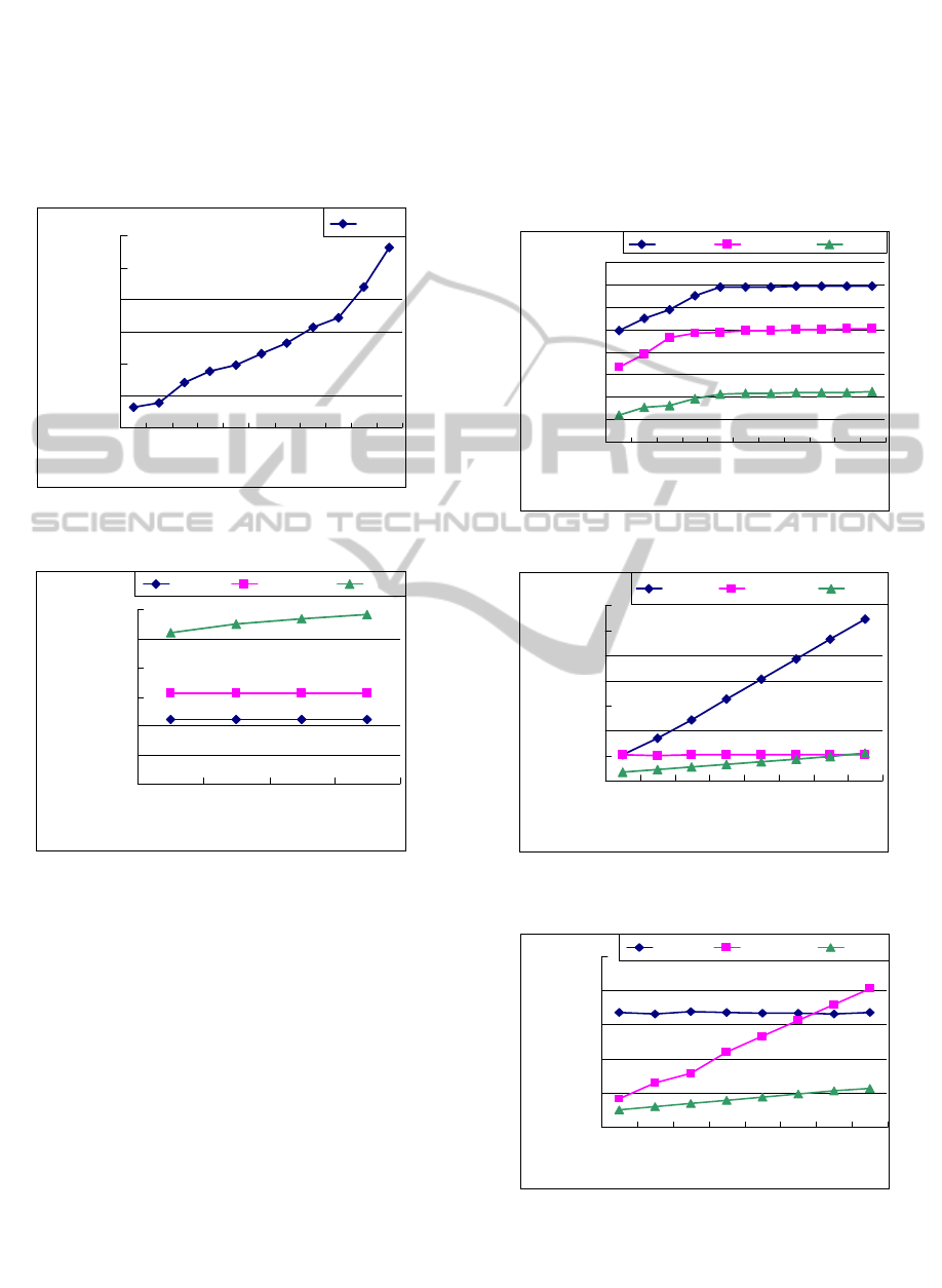
The memory usage of each algorithm is shown in

Figure 7. PPP uses more memory space because of

keeping the token list and the counter sequences for

the query records. Moreover, since the top-k pairs of

records, regarding the query records and the data

records of each time slot in the current window, are

kept as candidate results, AllTopk uses more

memory space than Naïve.

0.1

0.2

0.3

0.4

0.5

0.6

50 100 150 200 250 300 350 400 450 500 550

Query Size (records)

Preprocessing time (s)

PPP



Figure 6: Relation between Preprocessing time of PPP and

Query size.

100

1000

10000

100000

1000000

50 100 150 200

Query Size (records)

Memory Usage (Bytes)

Naive AllTopk PPP



Figure 7: Relation between Memory usage and Query size.

The experiment results on varying k are shown in

Figure 8. As can been seen, PPP still outperforms

AllTopk and Naïve in this experiment. The

experiment results on varying Window Size are

shown in Figure 9. As shown in Figure 9, the

processing time of AllTopk is quite stable and seems

not influenced by Window Size. This is because we

only concern about the data records arriving at the

last time slot rather than all of the data records

contained in the whole window as in Naïve.

Moreover, although the processing time of PPP

increases with the increasing of Window Size, the

increasing degree is lightweight. PPP is more

efficient than the others in most of the cases. The

experiment results on varying Sliding size are shown

in Figure 10. In this experiment, Time Slot Size is

randomly chosen from a range of [120, 140]. As

shown in Figure 10, the larger the value of Sliding

Size is, the longer the processing time of AllTopk

will be. This is because the number of data records

to be processed whenever the window slides

increases with the increasing of Sliding Size.

Moreover, as Naïve concerns the data records

contained in the current window, its processing time

is stable and not influenced by Sliding Size.

100

150

200

250

300

350

400

1 102030405060708090100

Processing Time (s)

Naive AllTo

k PPP

Figure 8: Relation between Processing time and k.

200

400

600

800

1000

1200

1400

12345678

Window Size (time slots)

Processing Time (s)

Naive AllTopk PPP

Figure 9: Relation between Processing time and Window

size.

100

200

300

400

500

12345678

Sliding Size (time slots)

Processing Time (s)

Naive AllTopk PPP

Figure 10: Relation between Processing time and Sliding

size.

OnContinuousTop-kSimilarityJoins



5 CONCLUSIONS

We make the first attempt to address the problem of

continuous top-k similarity joins in this paper. We

also propose two algorithms named AllTopk and

PPP to solve this problem. The AllTopk algorithm

computes the top-k pairs of records regarding the

data records arriving at the last time slot and the

query records to generate the candidate results. On

the other hand, in the PPP algorithm, the query

records are processed in advance to make each data

record able to be compared with all of the query

records at one time. The experiment results

demonstrate that PPP outperforms AllTopk and a

naïve algorithm. In the near future, we consider

solving another similar problem in the environment

of data streams, which takes into account two data

streams and continuously finds the top-k pairs of

records from these two data streams.

ACKNOWLEDGEMENTS

We thank the Taiwan Ministry of Economic Affairs,

Taiwan National Science Council, and Institute for

Information Industry (Fundamental Industrial

Technology Development Program 1/4) for

financially supporting this research.

REFERENCES

Arasu, A., Ganti, V., and Kaushik, R., 2006. Efficient

exact set-similarity joins. In Proceedings of the 32nd

International Conference on Very Large Data Bases,

VLDB2006. pp. 918-929.

Broder, A., Glassman, S., Manasse, M., and Zweig, G.,

1997 Syntactic clustering of the web. Computer

Networks, vol. 29, no. 8-13, (1997) pp. 1157-1166.

Bayardo, R., Ma, Y., and Srikant, R., 2007. Scaling up all

pairs similarity search. The 16th International World

Wide Web Conference, WWW2007, New York, NY,

USA, pp. 131-140.

Chowdhury, A., Frieder, O., Grossman, D., and McCabe,

M., 2002. Collection statistics for fast duplicate

document detection. ACM Trans. Inf. Syst., vol. 20, no.

2, (2002) pp. 171-191.

Chaudhuri, S., Ganti, V., and Kaushik, R., 2006. A

primitive operator for similarity joins in data cleaning.

In Proceedings of the 22nd International Conference

on Data Engineering, ICDE2006, Atlanta, Georgia.

Cohen, W., 1998. Integration of heterogeneous databases

without common domains using queries based on

textual similarity. In Proceedings of the ACM Special

Interest Group on Management of Data, SIGMOD1998,

New York, NY, USA, pp. 201-212.

Charikar, M., 2002. Similarity estimation techniques from

rounding algorithms. In Proceedings of the 34th Annual

ACM Symposium on Theory of Computing, STOC2002,

Montreal, Quebec, Canada, pp. 380-388.

Gionis, A., Indyk, P., and Motwani, R., 1999. Similarity

search in high dimensions via hashing. In Proceedings

of the 25th International Conference on Very Large

Data Bases, VLDB1999, Edinburgh, Scotland, UK, pp.

518-529.

Henzinger, M., 2006. Finding near-duplicate web pages: a

large-scale evaluation of algorithms. In Proceedings of

the ACM Special Interest Group on Information

retrieval, SIGIR2006, New York, NY, USA. pp.

284-291.

Sarawagi, S., and Bhamidipaty, A., 2002. Interactive

deduplication using active learning. ACM Special

Interest Group on Knowledge Discovery in Data,

KDD2002, New York, NY, USA, pp. 269-278.

Sarawagi, S., and Kirpal, A., 2004. Efficient set joins on

similarity predicates. In Proceedings of the ACM

Special Interest Group on Management of Data,

SIGMOD2004, New York, NY, USA, pp. 743-754.

Xiao, C., Wang, W., Lin, X., Shang, H., 2009. Top-k set

similarity joins. 25th International Conference on Data

Engineering. ICDE2009, Shanghai, China, pp.

916-927.

Xiao, C., Wang, W., Lin, X., and Yu, J. X., 2008. Efficient

similarity joins for near duplicate detection. In

Proceedings of the 17th International World Wide Web

Conference, WWW2008, New York, NY, USA, pp.

131-140.

DATA2012-InternationalConferenceonDataTechnologiesandApplications