
An Efficient Sampling Scheme for Approximate Processing of
Decision Support Queries
Amit Rudra
1
, Raj P. Gopalan
2
and N. R. Achuthan
3
1
School of Information Systems, Curtin University, Kent Street, Bentley, WA 6155, Australia
2
Department of Computing, Curtin University, Kent Street, Bentley, WA 6155, Australia
3
Department of Mathematics and Statistics, Curtin University, Kent Street, Bentley, WA 6155, Australia
Keywords: Sampling, Approximate Query Processing, Data Warehousing.
Abstract: Decision support queries usually involve accessing enormous amount of data requiring significant retrieval
time. Faster retrieval of query results can often save precious time for the decision maker. Pre-computation
of materialised views and sampling are two ways of achieving significant speed up. However, drawing
random samples for queries on range restricted attributes has two problems: small random samples may
miss relevant records and drawing larger samples from disk can be inefficient due to the large number of
disk accesses required. In this paper, we propose an efficient indexing scheme for quickly drawing relevant
samples for data warehouse queries as well as propose the concepts of database and sample relevancy ratios.
We describe a method for estimating query results for range restricted queries using this index and
experimentally evaluate the scheme using a relatively large real dataset. Further, we compute the confidence
intervals for the estimates to investigate whether the results can be guaranteed to be within the desired level
of confidence. Our experiments on data from a retail data warehouse show promising results. We also report
the levels of accuracy achieved for various types of aggregate queries and relate them to the database
relevancy ratios of the queries.
1 INTRODUCTION
Analytical queries containing aggregate functions
such as sum and average on a data warehouse are
used to gain a good sense of the business situation
and to support business decisions. Most often we
require timely retrieval of query results with an
acceptable level of accuracy rather than absolute
precision, and so approximate results within certain
limits of accuracy will be acceptable to the user. Pre-
computation with materialized views and sampling
are two ways to handle such queries. However, it is
impractical to maintain a large number of
materialized views for all possible combinations of
information retrieval (Hellerstein et al., 1997). In
contrast, sampling can provide faster results that are
accurate within given assured confidence levels.
The main motivation for use of sampling in
processing queries on a large database or a data
warehouse is to save time and resources. Even
though random sampling is both efficient and
effective as an approximation method, its use for
database querying has attracted significant research
interest only recently (Li et al, 2008); (Joshi and
Jermaine, 2008); (Jin et al., 2006). Sampling has
also been shown to be effective for aggregate
queries (Hellerstein et al., 1997); (Jermaine, 2007;
(Jin et al., 2006); (Jermaine, 2003); (Bernadino et
al., 2002); (Speigel and Polyzotis, 2009; Jermaine et
al., 2004). As sampling data may not be fully
representative of the entire data in a data warehouse,
it is desirable to return both the query result and the
confidence intervals that indicate the reliability of
the results (Li et al, 2008).
A significant problem with random sampling for
database queries from a database on stored disk is
that picking records at random requires almost the
same amount of I/O as processing the query over the
whole database (Olken and Rotem, 1990). To keep
down the cost of sampling based query processing, a
more efficient method of drawing samples is needed.
Another problem is that a random sample drawn
from a very large dataset may not contain relevant
records that satisfy the range restrictions of a given
query. To deal with this problem, we require a
sampling scheme that will include in the sample
16
Rudra A., Gopalan R. and Achuthan N..
An Efficient Sampling Scheme for Approximate Processing of Decision Support Queries.
DOI: 10.5220/0003995100160026
In Proceedings of the 14th International Conference on Enterprise Information Systems (ICEIS-2012), pages 16-26
ISBN: 978-989-8565-10-5
Copyright
c
2012 SCITEPRESS (Science and Technology Publications, Lda.)

records satisfying the query predicates.
Joshi and Jermaine (2008) introduced the ACE
Tree which is a binary tree index structure for
efficiently drawing samples for processing database
queries. They demonstrated the effectiveness of this
structure for single and two attribute database
queries, but did not deal with multi-attribute
aggregate queries. For extending the ACE Tree to k
key attributes, Joshi and Jermaine proposed binary
splitting of one attribute range after another at
consecutive levels of the binary tree starting from
the root; from level k+1, the process is repeated with
each attribute in the same sequence as before. This
process could lead to an index tree of very large
height for a data warehouse even if only a relatively
small number of attributes are considered.
Li et al. (2008) proposed a sampling cube
framework for answering analytical queries on a
data warehouse which calculates confidence
intervals for any multidimensional query. The
sampling cube is constructed from a random sample
of the data warehouse. After building the sampling
cube, there is no further access to the original data
records should a query require a different sample
from the one already drawn. If a query has too few
sample records in the sampling cube, they expand
the query to gather more sample records from the
sampling cube itself in an attempt to improve the
quality of the query result.
In this paper, we propose the k-MDI Tree which
extends the ACE Tree structure to deal with multi-
dimensional data warehouse queries. Unlike the
ACE Tree, the k-MDI tree allows non-binary splits
of data ranges for key values that do not split evenly
into 2
n
distinct ranges. The number of levels in the k-
MDI tree can be limited to the number of key
attributes. The shallow tree structure resulting from
multi-way branching also facilitates quicker retrieval
of leaf nodes from disk storage. Unlike the sampling
cube of Li et al. (2008), new samples that contain
relevant records are drawn for each query. These
records can be considered as drawn from a subset of
the data warehouse that satisfies the query
predicates. In estimating the query results, we take
into account the proportion of relevant records for
the query in the whole data warehouse. The
sampling and estimation methods are evaluated
experimentally using a real life data set.
The rest of the paper is organized as follows: In
Section 2, we define some relevant terms and briefly
describe the ACE Tree structure. In Section 3, our k-
way multi-dimensional (k-MDI) indexing structure
is described in detail. We also introduce the concept
of relevancy ratios, both for the database and a
specific sample. Section 4 reports the experimental
results that evaluate the efficacy of our scheme.
Section 5 is the conclusion of the paper.
2 TERMS, DEFINITIONS AND
ACE TREE STRUCTURE
In this section, we define some terms pertaining to
data warehousing, define confidence interval and
then review briefly the ACE Tree structure (Joshi
and Jermaine, 2008) that has preceded the k-MDI
tree we propose in Section 3.
2.1 Dimensions and Measure
To support decision support queries, data is usually
structured in large databases called data warehouses.
Typically, data warehouses are relational databases
with a large table in the middle called the fact table
connected to other tables called dimensions. For
example, consider the fact table Sales shown as
Table 1. A dimension table Store linked to StoreNo
in this fact table will contain more information on
each of the stores such as store name, location, state,
and country (Kimball and Moss, 2002). Other
dimension tables could exist for items and date. The
remaining attributes like quantity and amount are
typically, but not necessarily, numerical and are
termed measures. A typical decision support query
aggregates a measure using functions such as Sum(),
Avg() or Count(). The fact table Sales along with all
its dimension tables form a star schema.
Table 1: Fact table Sales.
SALES
Store
No
Date Item Quantity Amount
21 12-Jan-11 iPad 223 123,455
21 12-Jan-11 PC 20 24,800
24 11-Jan-11 iMac 11 9,990
77 25-Jan-11 PC 10 12,600
In decision support queries a measure is of
interest for calculation of averages, totals and
counts. For example, a sales manager may like to
know the total sales quantity and amount for certain
item(s) in a certain period of time for a particular
store or even all (or some) stores in a region. This
may then allow her to make decisions to order more
or less stocks as appropriate at a point in time.
AnEfficientSamplingSchemeforApproximateProcessingofDecisionSupportQueries
17

2.2 Confidence Interval
When estimating with samples we indicate the
reliability of the estimate by its confidence interval.
Consider a sample of records x with the mean of the
sample denoted by ̅, and the size of the sample n.
For a desired confidence level (e.g. 95%) the
confidence interval estimator of the population mean
µ
is given by:
̅ – t
α/2
√
, ̅ + t
α/2
√
where t
α/2
is the critical t-value and s the standard
deviation of the sample (Keller, 2009).
2.3 ACE Tree Structure
The ACE Tree is a balanced binary tree where the
leaf nodes contain the randomized samples of key
values and the internal nodes above them are the
index nodes. Each internal node contains a range R
of key values, a key value k that splits R into left and
right sub-trees, pointers to the left and right branch
(child) nodes, and counts of database records falling
in the left and right sub-trees. Figure 1 shows the
structure of an example ACE Tree. The root node I
1,1
with its range I
1,1
.R labeled as [0-64] signifies the
key value range of the whole data set. The key of the
root node partitions the range I
1,1
.R into I
2,1
.R = [0-
32] and I
2,2
.R = [33-64]. This partitioning of ranges
is propagated down the tree among the descendants
of respective nodes. The ranges associated with a
section of a leaf node are determined by the ranges
associated with each internal node on the path from
the root node to the leaf. If we look at the path from
I
1,1
i.e. the root node down to the leaf node L
4
, we
come across the following ranges 0-64, 0-32 and 17-
24. A leaf node is partitioned into sections (S
1
, S
2
,
…), their number depending on the number of
dimensions indexed. Thus, the first section L
4
.S
1
has
a random sample of records in the range 0-64; L
4
.S
2
has them in the range 0-32; L
4
.S
3
in the range 17-32
and L
4
.S
4
in the range 25-32. The size of each leaf is
chosen as the number of records that can be stored in
a disk block and so the number of leaf nodes
depends on the size of the database which also
determines the height of the index tree itself.
2.4 Sampling for a Query using the
ACE Tree
Referring to Figure 1, consider a query Q with a
range of [28-38]. The query execution algorithm
proceeds by traversing down I
1,1
, the root node. Both
I
2,1
.R and I
2,2
.R overlaps with Q.
Figure 1: Structure of the ACE Tree.
A level down from I
2,1
, only I
3,2
.R, overlaps with
Q. Traversing down to the leaf nodes, the algorithm
finds the right leaf node’s range [25-32] overlaps
with Q and so retrieves records from L
4
. The
relevant records in the query’s range are returned for
the sample which includes record 28 from L
4
.S
2
,
record 30 from L
4
.S
3
and records 29 and 31 from
L
4
.S
4
. Next, the algorithm traverses down the right
node I
2,2
below the root to the leaf node L
5
and
retrieves all relevant records from all sections of L
5
to the pool of sample records.
2.5 Extended ACE Tree for Multiple
Dimensions
Joshi and Jermaine (2008) proposed extending the
ACE Tree from a single dimension to multiple
dimensions as follows: Given key attributes
(dimensions), a
1
, ..., a
k
, split the range of values for
a
1
into two sub trees of approximately equal number
of keys below the root (level 1); for each node at
level 2, similarly perform a binary split of the range
of key values for a
2
and so on up to level k for
attribute a
k
. Then at level k+1, split the attribute
values of a
1
again followed by a
2
, etc. at further
lower levels.
In real life data, a dimension’s values may not
split evenly into 2
n
distinct ranges. For example, if a
dimension has an odd number of key values, say -
k
1
, k
2
and k
3
, with cardinalities of 30000 each; then,
we cannot split them evenly into 2 distinct ranges
but we can do so into 3. The height of the tree will
be very large even for a moderate sized data
warehouse with a relatively small number of
dimensions.
L
1
L
2
L
3
L
4
L
5
L
6
L
7
L
8
32
16
48
8
24
40
56
I
1,1
I
2
,
1
I
2
,
2
I
3
,
2
I
3
,
4
I
3,1
I
3,3
0-32
0-64
33-64
0-16 33-48
17-32
49-64
Index Nodes
(
circled numbers
indicate median,
quartile,… values)
Leaf
Nodes
23
62
45
19 30
25
18
15
6
29
31
26
27
28
0-64 0-32 17-32 25-32
L
4.
S
1
L
4.
S
2
L
4.
S
3
L
4.
S
4
Sections of a lea
f
node (
with sample
d
records showing thei
r
key values)
ICEIS2012-14thInternationalConferenceonEnterpriseInformationSystems
18

3 MULTIDIMENSIONAL
INDEXING
We propose the k-MDI tree which extends the ACE
Tree index for multiple dimensions while
overcoming the limitations of the ACE Tree
discussed in Section 2.5. The height of the k-MDI
tree is limited to the number of key attributes. As a
multi-way tree index, it is relatively shallow even for
a large number of key value ranges and so requires
only a small number of disk accesses to traverse
from the root to the leaf nodes.
3.1 k-ary Multidimensional Index
(k-MDI)
The k-ary multi-dimensional index tree (k-MDI tree)
is a k-ary balanced tree as described below:
1. The root node of a k-MDI tree corresponds to the
first attribute (dimension) in the index.
2. The root points to k
1
(k
1
≤ k) index nodes at level
2, with each node corresponding to one of the k
1
splits of the ranges for attribute a
1
.
3. Each of the nodes at level 2, in turn, points to up
to k
2
(k
2
≤ k) index nodes at level 3 corresponding to
k
2
splits of the ranges of values of attribute a
2
;
similarly for nodes at levels 3 to h, corresponding to
attributes a
3
,..., a
h
.
4. At level h, each of up to k
h-1
nodes points to up to
k
h
(k
h
≤ k) leaf nodes that store data records.
5. Each leaf node has h+1 sections; for sections 1 to
h, each section i contains random subset of records
in the key range of the node i in the path from the
root to the level h above the leaf; section h+1
contains a random subset of records with keys in the
specific range for the given leaf.
Thus, the dataset is divided into a maximum of k
h
leaf nodes with each leaf node, in turn, consisting of
h+1 sections and each section containing a random
subset of records. The total number of leaf nodes
depends on the total number of records in the dataset
and the size of a leaf node (which may be chosen as
equal to the disk block size or another suitable size).
More details on leaf nodes and sections are given in
Section 3.3. In real data sets, the number of range
splits at different nodes of a given level i need not be
the same. For convenience, the number of splits at
all levels are kept as k in Figure 2 that shows the
structure of the general scheme for k-MDI multilevel
index tree of attributes A
1
, A
2
, …, A
h
with k ranges
(R
11
, R
12
, …, R
1k
), (R
21
, R
22
, …, R
2k
), … (R
h1
, R
h2
, …,
R
hk
) respectively at levels (1, …,h).
An example of the k-MDI tree is shown in Figure
3 from a store chain dataset with three dimensions –
store, date sold and item number. The number of
range splits and hence branches from non-leaf nodes
vary between 2 and 4 in this example.
3.2 Leaf Nodes
Similar to the ACE tree structure, the lowest level
nodes of a k-MDI tree point to leaf nodes containing
data records. The data records are stored in h+1
sections, where h is the height of the tree. Section S
1
of every leaf node is drawn from the entire database
with no range restriction on the attribute values.
Each section S
i
(2 ≤ i ≤ h+1) in a leaf node L is
restricted on the range of key values by the same
restrictions that apply to the corresponding sub-path
along the path from the root to L. Thus for section
S
2
, the restrictions are the same as on the branch to
the node at level 2 along the path from the root to L
and so on.
Figure 3 shows an example leaf node projected
from the sample k-MDI tree. The sections are
indicated above the node with attribute ranges for
each section below the node. The circled numbers in
each section indicate record numbers that are
randomly placed in the section. The range
restrictions on the records are indicated below each
section, where the first section S
1
has records drawn
from the entire range of the database. Thus, it can
contain records uniformly sampled from the whole
dataset. The next section S
2
has restriction on the
first dimension viz. store (for leaf node L
7
this range
is store numbers 1-16). The third section S
3
has
restrictions on both first and second dimensions viz.
store and date. While the last section S
4
has
restrictions on all the three dimensions – store, date
and item.
The scheme for selection of records into various
leaf nodes and sections is explained in detail in the
following section.
3.3 Building the k-MDI Tree
The purpose of the k-MDI tree is to quickly retrieve
relevant random samples of records for processing
data warehouse queries. The records in the sample
are obtained from leaf nodes by traversing the index
from the root. The k-MDI Tree is built in the
following three steps:
1. First, the dataset records are sorted by the first
key attribute a
1
as the major field, followed by the
second attribute a
2
and so on until the last attribute
a
h
.
AnEfficientSamplingSchemeforApproximateProcessingofDecisionSupportQueries
19

2. The next step is to find the split points of key
attribute values in the index tree at the levels 1 to h
so that the number of records of the dataset that fall
under each sub-tree rooted at levels 2 to h is
approximately equal. The k
1
-1 split points at level 1
are chosen such that the total number of records in
the dataset are split into k
1
approximately equal
parts; the records falling under each of the nodes at
level 2 are split into k
2
approximately equal parts,
and so on until the records falling under each of the
nodes at level h split into k
h
approximately equal
parts. The number of splits at all the levels in the
index should be such that the number of leaf nodes
are equal to a pre-computed number based on the
total number of records in the dataset and the size of
each leaf node (which could be chosen as the disk
block size as in the case of the ACE Tree or some
other suitable size).
3. Next, a random number between 1 and h+1 is
assigned to each data record as its section number.
Depending on the section number and its composite
key value, the record is assigned to a leaf node as
follows: If the section number is 1, the record is
assigned randomly to any one of the leaf nodes in
the tree; if the section number is i (2≤i≤h), starting
from the root of the index tree, we locate the root of
a sub-tree at level i in which the key of the record
falls and assign the record randomly to section i of
any of the leaf nodes in that sub-tree;
if the record’s section number is h+1, it is assigned
to the specific leaf node where the record’s key
value belongs. When all the records have been thus
assigned section and leaf node numbers, the dataset
is re-organised with records sorted according to their
leaf node and section numbers.
3.4 Using the k-MDI Tree for Data
Warehouse Queries
By using a k-MDI tree index, we can draw stratified
samples for data warehousing queries from restricted
ranges of key values. In this section, we first
introduce two measures that are useful for the
estimation of query results using such samples. The
database relevancy ratio (DRR) of a query Q,
denoted by ρ(Q) is the ratio of the number of records
in a dataset D that satisfies the query conditions to
the total number of records in D. For a query with
no condition, ρ(Q) is 1. Similarly, the sample
relevancy ratio (SRR) of a query Q for a sample set
S, denoted by ρ(Q, S) is defined as the ratio of the
number of records in S that satisfy a given query Q
to the total number of records in S.
In a true random sample of records, the SRR for
a query Q is expected to be equal to its DRR, i.e.,
E(ρ(Q, S) ) = ρ(Q). A sample with ρ(Q, S) > ρ(Q) is
likely to give a better estimate of the mean than a
true random sample. However, for the sum of a
column, the sample needs to be representative of the
population, i.e., ρ(Q, S) should be close to ρ(Q).
Consider the following formula for estimating
the sum (Berenson and Levine, 1992):
=̂
,
where N is the cardinality of the population, ̂ the
estimated proportion of records satisfying the query
conditions and
the mean of records in the sample
satisfying the query condition. In order to estimate
the mean we can use all relevant sampled records
from all sections of the retrieved leaf nodes, but to
estimate the sum we can use sampled records
Figure 2: General structure of the k-MDI tree – A
1
, A
2
, …, A
h
are h attributes and R
ij
the i-th attribute’s j-th range high
water mark (HWM).
A
1
A
2
. . .
A
h
R
11
R
12 . . .
R
1k
Leaf nodes
. . .
Index tree
A
1
A
2
... A
h-1
A
h
R
11
R
21
R
h-1 1
R
h1
R
h2 …
R
hk
A
1
A
2
... A
h
R
11
R
21
R
22 …
R
2k
A
1
A
2
... A
h
R
12
R
21
R
22 …
R
2k
A
1
A
2
... A
h
R
1k
R
21
R
22 …
R
2k
... ... .... . .
.
.
.
.
.
.
. . .
A
1
A
2
... A
h-1
A
h
R
11
R
21
R
h-1 2
R
h1
R
h2 …
R
hk
. . .
A
1
A
2
... A
h-1
A
h
R
1k
R
2k
R
h-1 k
R
h1
R
h2 …
R
hk
...
...
... ...
. . .
...
Level 1-Dim A
1
Level 2-Dim A
2
Level h-Dim A
h
.
.
ICEIS2012-14thInternationalConferenceonEnterpriseInformationSystems
20

only from section S
1
, which is the only section with
records drawn randomly from the entire dataset. For
estimating the sum for a query with conditions on
some of the indexed dimensions we use appropriate
sections of the retrieved leaf nodes to get a better
estimate of the mean; the records from section S
1
are
also used to get a fair estimation of the proportion
records that satisfy the query conditions.
3.5 Effect of Sectioning on Relevancy
Ratio
As discussed earlier, sections S
1
to S
h+1
of each leaf
node contain random collections of records with the
difference that S
1
contains records from the entire
dataset while other sections contain random records
from restricted ranges of the key attributes. Consider
a query with the same range restrictions on all three
dimensions (store, date and item) as section L
7
.S
4
in
Figure 3. We are then likely to get more relevant
records in the sample from the second section L
7
.S
2
than from S
1
since records of S
2
have restrictions on
the first dimension of store that matches the query
condition. Records in S
3
will have restrictions on
both store and date dimensions that match that of the
query and so are likely to contain more relevant
records than in S
2
. All records in section L
7
.S
4
will
satisfy the query since the range restrictions on S
4
exactly match the query. Mathematically, for a query
Q having restrictions as mentioned above:
ρ(Q) = E(ρ(Q, L
7
.S
1
)) ≤ E(ρ(Q, L
7
.S
2
))
≤ E(ρ(Q, L
7
.S
3
)) ≤ E(ρ(Q, L
7
.S
4
))
Using this property of the k-MDI tree, it is possible
to quickly increase the size of a sample that is too
small, by including more records from other sections
of the retrieved leaf nodes.
3.6 Record Retrieval to Process a
Query
The objective of using the k-MDI tree is to retrieve a
significant number of relevant records (i.e. records
that satisfy the query conditions) in the sample
drawn for processing a given query. The query
conditions may span sections of one or more leaf
nodes which can be reached from index nodes that
straddle more than one range of attribute values.
These leaf nodes can be accessed by traversing the
tree from the root using the attribute value ranges in
the query conditions and sections from multiple leaf
nodes can be combined to form the sample.
We describe the retrieval process using an
example query on the sample database of Figure 4.
Consider a query Q
0
about sales in store 12 for date
range 1-13 and item range 12M-20M. The retrieval
algorithm finds the sections of leaf nodes for this
query as follows:
1. Search index level 1 to locate the relevant store
range. Store 12 is in the left most range of 1-16.
2. Traverse down to index level 2 (date), indicated
by a dashed arrow in Figure 4, along the first store
range. Since there is a condition on date (1-13),
compare the HWMs (high water marks) of the three
ranges and find that it fits into two date ranges viz.
the first and the second. Make a note of these date
ranges.
3. Traverse down using the first date range to the
next index level which has item ranges. Since there
is a condition on item numbers (12M-20M),
compare this range with HWMs and find that it fits
into two ranges viz. the third and the fourth. Make a
note of these item ranges.
4. Traverse down using the third item range to
relevant leaf pages and make a note of them.
5. Iterate step 4, except this time using the fourth
item range.
6. Next, repeat the above three steps i.e. steps 3
through 5; but this time using the second date range
instead.
7. Now retrieve records from the relevant sections
in the four leaf nodes (viz. L
3
, L
4
, L
7
and L
8
) to form
a sample for the given query.
3.7 Estimating Query Results from
Samples
In decision support queries on large databases, the
most common estimation performed is either of the
mean or the sum of a column measure (Jin et al.,
2006). We maintain a table representing a histogram
of record counts for each leaf node and its sections.
It is used to estimate the number the leaf nodes
required to have adequate number of samples. The
following steps outline our method of estimating the
mean, sum, standard deviation and the confidence
intervals:
1. Draw a sample set L of leaf nodes as described in
Section 3.6 for the given sampling rate.
2. The following parameters are computed:
a. Sample size – n
b. Count of sampled records satisfying the
query condition – m
c. Count of records in all sampled S
1
sections of L
– n′
d. Count of records in all sampled
S1
sections of
AnEfficientSamplingSchemeforApproximateProcessingofDecisionSupportQueries
21
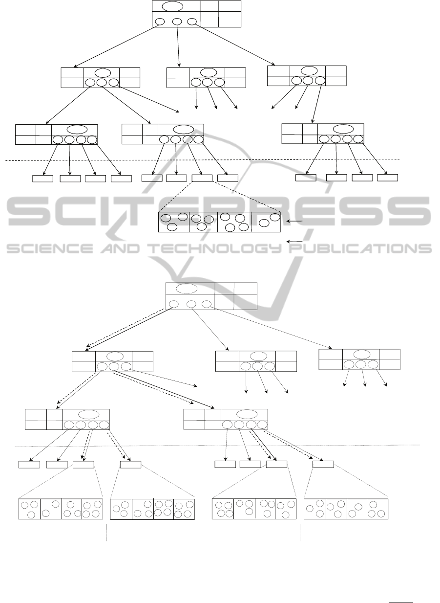
Figure 3: A leaf node (changes in range values for attributes are indicated in bold).
Figure 4: Navigation down index tree nodes for conditions on three dimensions.
L satisfying the query condition – m′
e. Sum of attribute (variable) value of all m
records – sum
f. Sum of squares of attribute value of the all
abovementioned m′ records – ′
g. The average sum of squares - Z =
́
Store# Item#
1 – 60 1 – 31 1M-21M
16 4 1 6 0
Date
Store# Item#
1 – 16 1 1 20 3 1 1
M-21M
Date
1 - 16
1 - 11 12 -20
Store#
Item#
1 – 16 1 – 11
7M
10M 15M 21M
Date
L
1
L
2
L
3
L
4
L
7
.S
1
St ore #: 1-60 1-16 1-16 1-16
Dat e: 1 -31 1-31 12-20 12-20
Ite m# : 1 M-21M 1M-21 M 1M-21 M 11M-15M
17
23
2
10
99
33
76
15
87
52
7
88
1M–7M
Level 1 index
(Store)
Level 2 index
(Date)
Level 3 index
(Item)
Leaf nodes
L
7
.S
2
L
7
.S
3
L
7
.S
4
Sections of a leaf node
Attribute ranges
I
1,1
I
2
,3
I
2,1
I
3,1
Store# Item#
17 – 4 1 11 20 31 1
M-21M
Date
I
2,2
Store# Item#
42 – 60 11 20 3 1 1
M-21M
Date
21 - 31
17-41 42 -60
8M–10M 11M–15M16M–21M
Store#
Item#
1 – 16 12 – 20
7M
10M 15M 21M
Date
L
5
L
6
L
7
L
8
1M–7M
I
3,2
8M–10M 11M–15M 16M–21M
. . . . . . . . . . . . . . . . . .
. . . . . . . . .
. . . . . . . . .
Store#
Item#
42 – 60 2 1 – 3 1
7M
10M 15M 21M
Date
L
33
1M–7M
I
3,9
8M–10M 11M–15M 16M–21M
L
34
L
35
L
36
21 -31
Store# Item#
1 – 60 1 – 31 1M-21M
16 41 60
Date
Store# Item#
1 – 16 11 20 31 1
M-21M
Date
Store#
Item#
1 – 16 1 – 11
7M
10M 15M 21M
Date
L
1
L
2
L
3
L
4
L
3
.S
1
Store#: 1-60 1-16 1-16 1-16 1-60 1-16 1-16 1-16 1-60 1-16 1-16 1-16 1-60 1-16 1-16 1-16
Date: 1-31 1-31 1-11 1-11 1-31 1-31 1-11 1-11 1-31 1-31 12-20 12-20 1-31 1-31 12-20 12-20
Item#:
1M-21M 1M-21M 1M-21M 11M-15M 1M-21M 1M-21M 1M-21M 16M-21M 1M-21M 1M-21M 1M-21M 11M-15M 1M-21M 1M-21M 1M-21M 16M-21M
17
23
8
L
3
.S
2
L
3
.S
3
L
3
.S
4
I
1,1
I
2
,3
I
2,1
I
3,1
Store# Item#
17– 41 11 20 31 1M-21M
Date
I
2,2
Store# Item#
42 – 60 11 20 31 1M-21M
Date
Store#
Item#
1 – 16 12 –20
7M
10M 15M 21M
Date
L
5
L
6
L
7
L
8
I
3,2
. . . . . .
. . .
7
2
21
55
73
22
43
L
4
.S
1
48
3
26
L
4
.S
2
L
4
.S
3
L
4
.S
4
32
44
56
69
63
92
93
52
43
20
28
L
7
.S
1
17
5
L
7
.S
2
L
7
.S
3
L
7
.S
4
39
95
70
25
L
8
.S
1
40
L
8
.S
2
L
8
.S
3
L
8
.S
4
88
74
41
. . . . . . . . .
. . . . . .
. . .
91
47
18
79
75
89
80
30
60
50
77
81
59
19
73
29
ICEIS2012-14thInternationalConferenceonEnterpriseInformationSystems
22

3. Estimating the sum, average, variance and C.I.
limits (Chaudhuri and Mukherjee, 1985):
a. Estimate of the number of records M that
satisfy the query condition in the population
(given the cardinality of the dataset N)
=
b. Estimate of Average ̅ =
c. Estimate of Sum
=
̅
d. Estimate of variance of Average v(
)
e. Confidence interval lower limit
f. Confidence interval upper limit
4 EXPERIMENTAL RESULTS
To evaluate the effectiveness of our sampling
technique based on the k-MDI tree, we performed
experiments on real life supermarket retail sales data
(TUN, 2011) for a month from 150 outlets. The data
warehouse is structured as a star schema shown in
Figure 5, with the fact table (itemscan) consisting of
over 21 million rows and three dimension tables viz.
storeInfo, itemDesc and storeMemberVisits. TPC-H
queries (TPC Benchmarks, 2011) with suitable
modifications for this sample data warehouse were
used in the experiments. Most of the TPC-H queries
involve SQL aggregate functions of sum(), avg() or
count(). A few include min() and max() which are
not easily calculated by sampling (Joshi, 2008;
Hellerstein et al., 1997). So, we investigated only
sum, avg and count in our experiments. The index
tree structure was simulated using the Oracle
DBMS. We clustered the fact table on leaf and
section number to maintain the records in that
sequence. This organisation supported the
simulation of both the storage and retrieval of
records for the experiments.
A set of three queries were used containing the
SQL functions – avg(), sum(), count() with varying
database relevancy ratios (DRR). The queries were
of the form:
Select Avg(totscanAmt), Sum(totscanAmt),
Count(*)
From itemscan, storeinfo, itemdesc
Where storeno between s1 and s2
And itemscan.storeno=storeinfo.storeno
And itemscan.itemno=itemdesc.itemno
And datesold between d1 and d2
And itemno between i1 and i2;
The DDR value was set high or low for the queries
by choosing a given proportion of the dimension
range for the query. For example, assuming a
uniform distribution of values for a dimension in the
database, we can get a DRR of approximately 0.33
on a single dimension query, by picking a third of
the dimension range. However, in practice we
empirically varied the dimension ranges in the
queries to get the desired DRR values.
The first test query had a condition on a single
dimension and a high DRR value of 0.37; the second
query had a lower DRR (0.05) with conditions on
two dimensions; and the third query had a very low
DRR (0.002) with conditions on all three
dimensions. The relevance of DRR in estimating the
query results may be seen from the query result
estimation process of Section 3.7. In step 3a, the
count
directly depends upon the DRR, which is
the statistical proportion p whose estimate is given
by
. In step 3c, the estimation of sum depends
on the count
and thereby on p.
We conducted the experiments using several
random samples at sampling rates of (1% - 12%) and
the results were averaged for each sampling rate.
The error for the three aggregate functions viz. avg,
sum and count were computed as the absolute value
of the difference between estimated and actual
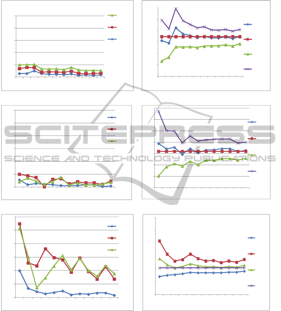
values for the whole database. Figure 6 shows the
results with error rates for both average (mean) of
totscanamt column, sum of totscanamt and count for
the different database relevancy ratios mentioned
above.
There are two graphs for each level of DRR.
Figure 6a shows the error rates for the average, the
sum of scan amount and count for high DRR. Figure
6b shows the confidence intervals (lower and upper
limits) for the average amount for high DRR. Figure
6b also shows the estimated and actual values of the
average scan amount. Figures 6c and 6d show
similar information as above for the low value of
DRR; Figures 6e and 6f show similar information
for very low DRR.
It is seen that for the high DRR query with ρ(Q
1
)
= 0.37, the error rates for the count, average and the
sum of the total scan amount stabilize as the
sampling rate is increased. The estimates are close
1
1
−
′
−
′
n
m
N
m
sum
))((
)1(
ˆ
ˆ
2
xZ
mM
mM
−
−
−
=
)1(
)(
)1(
)1(
1
1
−
′
′
−
′
−
′
−
′
−
−
′
−
′
=
n
mn
nn
m
Z
n
m
)1(
)(
)1(
)1(
1
1
−
′
′
−
′
−
′
−
′
+
−
′
−
′
=
n
mn
nn
m
Z
n
m
AnEfficientSamplingSchemeforApproximateProcessingofDecisionSupportQueries
23
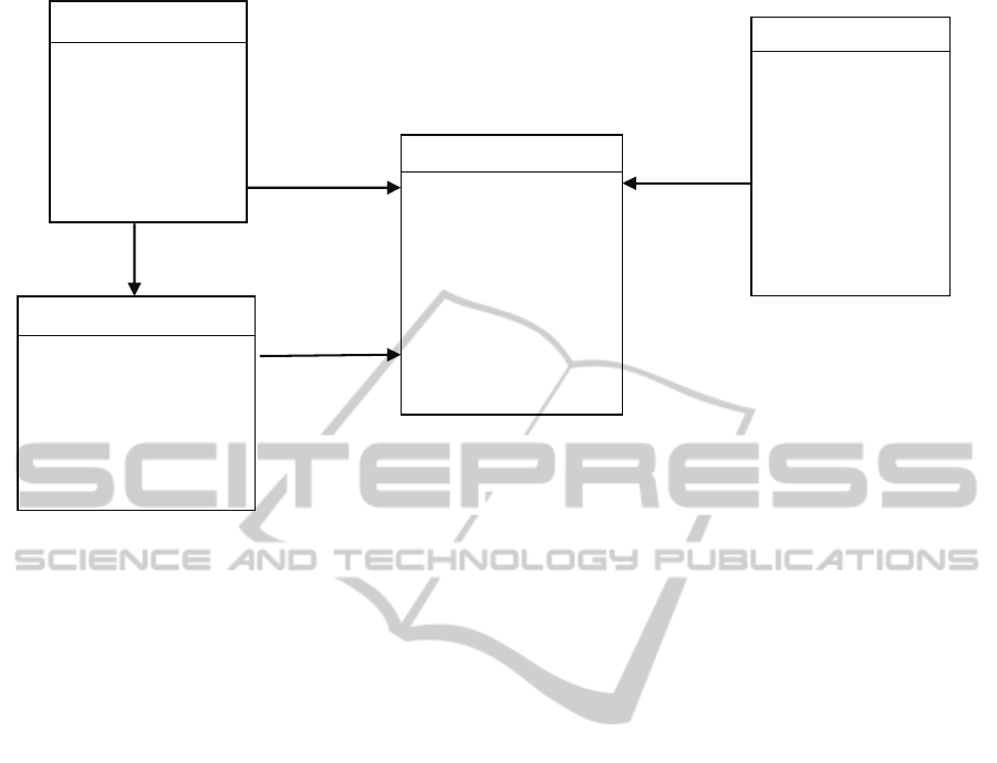
Figure 5: The schema for experimental retail sales data warehouse.
to the actual values for the lowest to the highest
sampling rates used and the true value of average is
always within the estimated confidence interval. For
the medium DRR query with ρ(Q
1
) = 0.05, we still
get error rates below the normally acceptable rate of
5%. For query with very low DRR of ρ(Q
1
) = 0.002,
the error rates for the average scan amount, for all
but 1% sampling rate, are below 5% and the true
values within the C.I. limits. But the error rates for
the estimated sum of scan amount and count of
records are not below the acceptable limit at any
sampling rate used for the very low DRR query.
Thus, we cannot satisfactorily estimate the sum and
the count for low values of DRR, while for medium
to high values of DRR the estimations of both the
sum and average are within acceptable error limits.
Also, it’s observed from the graphs that there is an
apparent close correlation between the estimates of
sum and count.
Time Improvement – Figure 7 shows the average
time for processing the queries at various sampling
rates and also the average time for processing these
queries on the full database. It is seen that there is a
significant time improvement from using the
sampling scheme.
5 CONCLUSIONS
In this paper, we proposed the k-MDI tree
indexwhich can be used to draw samples quickly for
answering multi-dimensional aggregate queries from
a data warehouse. The k-MDI tree extends the ACE
binary tree as a multi-way tree index. The maximum
number of levels of the k-MDI index is limited to the
number of key attributes and so makes the access to
the leaf nodes much quicker compared to a binary
tree index on external storage.
We also proposed the concepts of database
relevancy ratio (DRR) and sample relevancy ratio
(SRR) for queries. We investigated the effect of the
DRR on the accuracy of query results estimated
from samples drawn using the k-MDI index. From
the experimental evaluation of the sampling scheme
on a large real dataset, it is found that even at
relatively low sampling rates of 1% to 12 %, query
results can be estimated accurately with a minimum
of 95% confidence for queries with medium to high
DRR. At a very low DRR of 0.002, the estimated
values of sum and count fell outside the acceptable
confidence level of 95%, but the estimated mean
was within the 95% confidence interval even at very
low DRR. Depending on the sampling rate, the
sampling based query processing was on average 9
to 30 times faster than processing the same queries
against the whole dataset.
As future work, it is proposed to develop a
generic tool that can be used with some parameter
inputs to set up the k-MDI tree index for any data
warehouse schema. We also plan to further evaluate
the sampling based estimation scheme on data
warehouses with larger dimensions.
ITEMSCAN
storeno
datesold
itemno
visitno
qty
totalScanAmt
unitcost
unitprice
21,421,663
ITEMDESC
itemno
categoryno
subcategoryno
primarydesc
secondarydesc
colour
sizedesc
statuscode
:
19,825
STOREINFO
storeno
storename
regionno
districtno
storetype
address
:
150
STOREMEMBERVISTS
memberno
visitno
storeno
memberstatuscode
:
218,872
ICEIS2012-14thInternationalConferenceonEnterpriseInformationSystems
24
(a) Error rates for query with condition on one dimension (high
relevancy ratio).
(b) Confidence interval (AVG amt) for query with condition on
one dimension (high DRR).
(c) Error rates for query with condition on two dimensions
(medium relevancy ratio).
(d) Confidence interval (AVG amt) for query with condition on
two dimensions (medium DRR).
(e) Error rates for query with condition on three dimensions (low
relevancy ratio).
(f) Confidence interval for query with condition on three
dimensions (low DRR).
Figure 6: Error rates of average scan amount and sum of scan amount and confidence interval of average scan amount at
various sampling rates for high, medium and low relevancy ratios.
0
5
10
15
20
25
123456789101112
Error rate (%)
Sampling rate (%)
Error rates - Average, Sum & Count
Err rate
Count
Err Rate
Sum Amt
Err Rate
Avg Amt
24
24.5
25
25.5
26
26.5
27
123456789101112
Avg Amt
Sampling rate (%)
Average amount and C.I. Limits - High DRR
Estimate of
AvgAmt
Actual Avg
Amt
C.I.Lwr
Limit Avg
Amt
C.I.Upper
Limit Avg
Amt
0
5
10
15
20
25
30
123456789101112
Error rate (%)
Sampling rate (%)
Error rates Avg, Sum & Count
Err Rate
Avg Amt
Err Rate
Sum Amt
Err rate
Count
22
23
24
25
26
27
28
29
123456789101112
Value
Sampling rate (%)
C.I. Limits for Avg Amt, Actual vs Estimate
Estimat
e of
AvgAmt
Actual
Avg Amt
C.I.Lwr
Limit
Avg Amt
C.I.Uppe
r Limit
Avg Amt
0
5
10
15
20
25
30
123456789101112
Error rate (%)
Sampliing rate (%)
Error rates - Average, Sum & Count
Err Rate
Avg Amt
Err Rate
Sum Amt
Err rate
Count
15
17
19
21
23
25
27
123456789101112
Avg Amt
Sampling rate (%)
Average amount and C.I. Limits - Low DRR
C.I.Lower
Limit
C.I.Upper
Limit
Estimate
of Avg
Amt
Actual
Avg Amt
AnEfficientSamplingSchemeforApproximateProcessingofDecisionSupportQueries
25
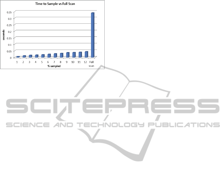
Figure 7: Query times at different sampling rates as
compared to full database scan.
REFERENCES
Berenson, M. L., Levine, D. M., 1992. Basic Business
Statistics - Concepts and Applications. Prentice Hall,
Upper Saddle River, New Jersey, USA.
Bernardino, J., Furtado, P., Madeira, H., 2002.
Approximate Query Answering Using Data
Warehouse Striping. Journal of Intelligent Information
Systems. 19:2, pp.145-167.
Chaudhuri, A., Mukherjee, R., 1985. Domain Estimation
in Finite Populations. Australian Journal of Statistics.
Vol. 27:2, pp. 135-137.
Hellerstein, H, Haas, P, Wang, J., 1997. Online
Aggregation. SIGMOD 1997, pp. 171-182.
Hobbs, L., Hillson, S., Lawande, S., 2003. Oracle9iR2
Data Warehousing. Elsevier Science, MA, USA.
Jermaine, C., 2007. Random Shuffling of Large Database
Tables. IEEE Transactions on Knowledge and Data
Engineering. 18:1, pp.73-84.
Jermaine, C., 2003. Robust Estimation with Sampling and
Approximate Pre-Aggregation. VLDB Conference
Proceedings 2003, pp. 886-897.
Jermaine, C., Pol, A., Arumugam, S., 2004. Online
Maintenance of Very Large Random Samples.
SIGMOD Conference Proceedings 2004.
Jin, R., Glimcher, L, Jermaine, C, Agrawal, G., 2006. New
Sampling-Based Estimators for OLAP Queries.
Proceedings of the 22
nd
International Conference on
Data Engineering (ICDE'06), Atlanta, GA, USA.
Joshi, S., Jermaine, C., 2008. Materialized Sample Views
for Database Approximation, IEEE Transactions on
Knowledge and Data Engineering, 20:3 pp. 337-351.
Keller, G., 2009. Statistics for Management and
Economics. Cengage Learning, Mason, OH, USA.
Kimball, R., Ross, M., 2002. The Data Warehouse
Toolkit: The Complete Guide to Dimensional
Modeling, 2nd Ed. John Wiley & Sons, Indianapolis,
USA.
Li, X., Han, J., Yin, Z., Lee, J-G., Sun, Y., 2008.
Sampling Cube: A Framework for Statistical OLAP
over Sampling Data. Proceedings of ACM SIGMOD
International Conference on Management of Data
(SIGMOD'08), Vancouver, BC, Canada, June.
Olken, F., Rotem, D., 1990, Random Sampling from
Database File. In: A Survey. International Conference
on Scientific and Statistical Database Management,
1990. pp. 92-111.
Spiegel, J., N. Polyzotis, 2009. TuG Synopses for
Approximate Query Answering. ACM Transactions on
Database Systems. (TODS) 34(1).
TPC Benchmarks, 2011. Transaction Processing
Performance Council - TPC-H: Decision Support
Benchmark. http://www.tpc.org [Accessed 20
November 2011].
TUN - Teradata University Network, 2011.
http://www.teradata.com/TUN_databases. [Accessed:
13 April 2007].
ICEIS2012-14thInternationalConferenceonEnterpriseInformationSystems
26
