
Visual Servoing Path-planning with Spheres
Tiantian Shen and Graziano Chesi
Department of Electrical and Electronic Engineering, University of Hong Kong, Pokfulam, Hong Kong
Keywords:
Sphere, Path-planning, Visual Servoing.
Abstract:
This paper proposes a path-planning approach for visual servoing in the case where the observed object fea-
tures are points and spheres. Two main situations are considered. In the first situation, it is supposed that at
least two points and at least a sphere are observed. In the second situation, it is supposed that at least three
spheres are observed. The problem consists of planning a trajectory in order to ensure the convergence of
the robot end-point to the desired location while satisfying visibility and workspace constraints, in particular
including occlusion and collision avoidance. A solution based on polynomial parametrizations is proposed
in order to determine a feasible path in the 3D space, and such a path is then followed by tracking its image
projection through image-based visual servoing. Some simulation results illustrate the proposed approach.
1 INTRODUCTION
Visual servoing is a technique which uses visual in-
formation to control the robot moving to a desired
location. Classical methods include image-based vi-
sual servoing (IBVS) (Hashimoto et al., 1991) and
position-based visual servoing (PBVS) (Taylor and
Ostrowski, 2000). They have well documented weak-
nesses and strengths (Chaumette, 1998b). In order to
better satisfy constraints that arise in visual servoing,
combination of IBVS and PBVS is explored such as
2 1/2-D visual servoing (Malis et al., 1999), partition
of the degrees of freedom (Oh and Allen, 2001) and
switched controllers (Gans and Hutchinson, 2007;
Chesi et al., 2004). Other approaches include: nav-
igation functions (Cowan et al., 2002), circular-like
trajectories for global convergence (Chesi and Vi-
cino, 2004), path-planning techniques (Mezouar and
Chaumette, 2002a; Chesi and Hung, 2007; Chesi,
2009; Shen and Chesi, 2012), omnidirectional vision
systems (Tatsambon Fomena and Chaumette, 2008),
and etc. See also the survey papers (Chaumette and
Hutchinson, 2006; Chaumette and Hutchinson, 2007)
and the book (Chesi and Hashimoto, 2010) for more
details.
In most of the literature, pixel coordinates of rep-
resentational points are the dominant visual features
used in a controller. On the other hand, other fea-
tures more intuitive than points, such as image mo-
ments (Chaumette, 2004; Tahri and Chaumette, 2005;
Tatsambon Fomena and Chaumette, 2008) and lu-
minance (Collewet and Marchand, 2010), have been
explored in a small part of the literature. Among
these works, solid objects that are more natural than a
point, such as circle, sphere and cylinder (Chaumette,
1998a), are considered as targets in visual servo-
ing. In particular, in the work of (Tatsambon Fom-
ena and Chaumette, 2008), a set of three-dimensional
(3-D) features are computed from image moments
of a sphere and used in a classical control law that
is proved to be globally asymptotically stable in the
presence of modeling errors and locally asymptot-
ically stable in the presence of calibration errors.
These 3-D features are structured through spherical
projection of the sphere, and therefore they are appli-
cable to omnidirectional vision systems. In this ref-
erence, however, high-level control strategies, such as
path-planning techniques, are not considered to take
into account constraints.
Thoughomnidirectional vision systems are not the
concern in this paper like what is considered in ref-
erence (Tatsambon Fomena and Chaumette, 2008),
however, sphere is our common interest as a target.
This paper aims to use path-planning techniques to
achieve a variety of constraints that arise in visual ser-
voing from spheres. A sphere may provide at most
three independent features, and therefore we combine
the sphere with at least two points or at least two other
spheres to constitute the whole target. Consequently,
two main situations are considered in this paper: a
sphere with two points and three spheres. For each of
the cases, constraints that are expected to be satisfied
include field-of-view limit of the whole target (which
contains at least one sphere), occlusion avoidance
22
Shen T. and Chesi G..
Visual Servoing Path-planning with Spheres.
DOI: 10.5220/0003998000220030
In Proceedings of the 9th International Conference on Informatics in Control, Automation and Robotics (ICINCO-2012), pages 22-30
ISBN: 978-989-8565-21-1
Copyright
c
2012 SCITEPRESS (Science and Technology Publications, Lda.)
among all the entities that consist of the target, and
collision avoidance between the camera and an given
obstacle in workspace. A camera path that meets
all these constraints is planned based on polynomial
parametrizations, and such a path is then followed by
tracking its image projection through image-based vi-
sual servoing. Some simulation results illustrate the
proposed approach.
The paper is organized as follows. Section II in-
troduces the notation and image moments of a sphere.
Section III presents the proposed strategy for visual
servoing path-planning with spheres. Section IV
shows some simulation results. Lastly, Section V con-
cludes the paper with some final remarks.
2 PRELIMINARIES
We denote by R the real number set, I
n×n
the n ×n
identity matrix, e
i
the i-th column of 3×3 identity ma-
trix, 0
n
the n×1 null vector, [v]
×
the skew-symmetric
matrix of v ∈R
3
.
2.1 Frame Transformation
Given two camera frames F
1
= {R
1
,t
1
} and F
2
=
{R
2
,t
2
} as shown in Fig. 1, the pose transformation
from F
1
to F
2
is expressed as {R,t}:
(
R = R
1
⊤
R
2
t = R
1
⊤
(t
2
−t
1
).
(1)
Suppose in the camera frame F
1
there is a 3D point
with its coordinates expressed as H, then the coordi-
nates of H in the camera frame of F
2
is R
⊤
(H −t).
Image projection of this point in F
2
is denoted as
[X,Y,1]
⊤
= KR
⊤
(H − t), where K ∈ R
3×3
is the
camera intrinsic parameters matrix.
Figure 1: Transformation between two camera frames.
2.2 Projection of a Sphere
In particular, when the target contains a sphere with
o = [x
o
,y
o
,z
o
]
⊤
as its center coordinates expressed in
the camera frame and r as its radius:
Figure 2: Projection of a sphere on the image plane.
(x−x
o
)
2
+ (y−y
o
)
2
+ (z−z
o
)
2
= r
2
, (2)
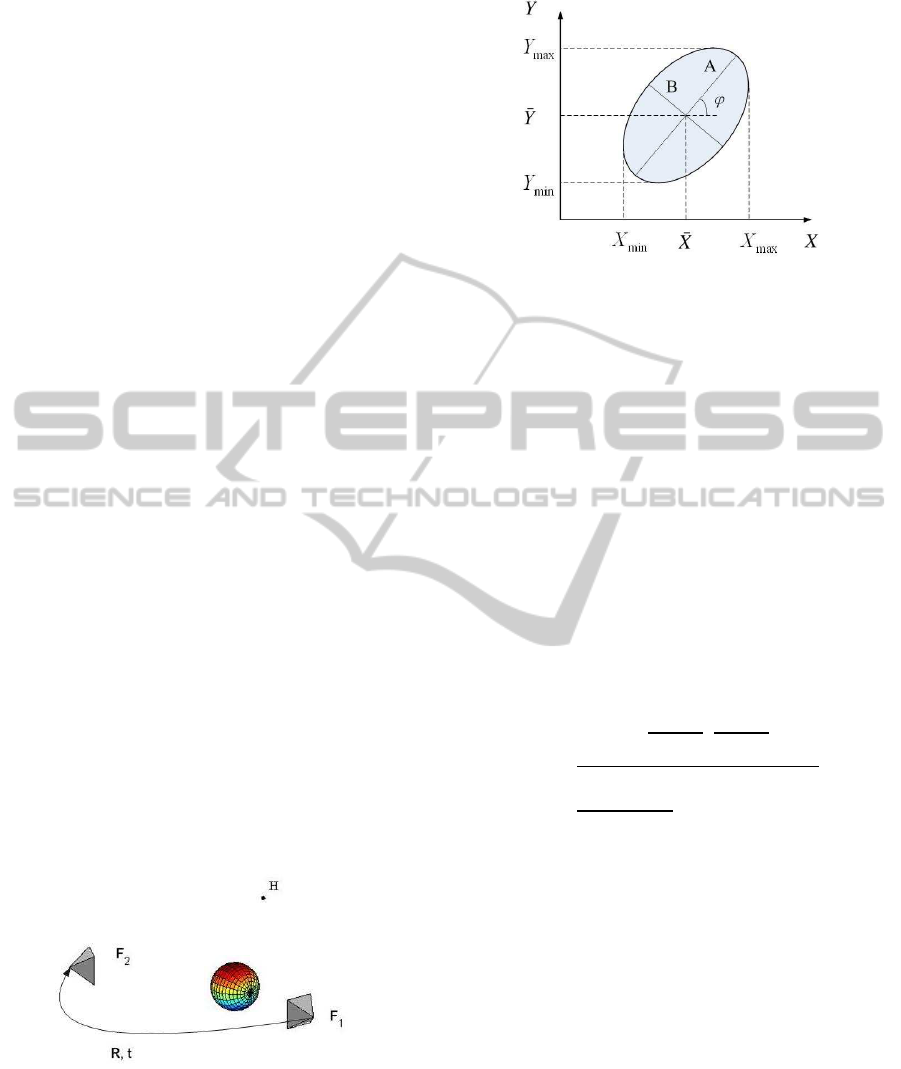
image projection of the sphere in the same camera
frame is in the form of an ellipse, the shape of which
consists of a set of points:
X(φ) =
¯
X + Acos(φ)cos(ϕ) −Bsin(φ)sin(ϕ),
Y(φ) =
¯
Y + Acos(φ)sin(ϕ) + Bsin(φ)cos(ϕ),
(3)
where φ ∈ (0, 2π], (
¯
X,
¯
Y) is the centroid of the ellipse,
A and B are half values of the major and minor diam-
eters, and ϕ describes the angle between the X-axis
and the major axis of the ellipse as shown in Fig. 2.
We induce the following relationship from results of
(Chaumette, 1998a), assuming pixels in the image are
in the shape of squares and f is the focal length of the
camera:
(
¯
X,
¯
Y,1)
⊤
= K
x
o
z
o
z
2
o
−r
2
,
y
o
z
o
z
2
o
−r
2
,1
⊤
,
A = f
q
r
2
(x
2
o
+ y
2
o
+ z
2
o
−r
2
)/(z
2
o
−r
2
),
B = f
q
r
2
/(z
2
o
−r
2
),
ϕ = arccos(y
o
/x
o
).
(4)
Suppose that I(X,Y) are pixel intensities of the el-
lipse area in a grey-scale image, raw image moments
m
ij
and central image moments µ
ij
of the pertinent
sphere are defined as:
m
ij
= Σ
X
Σ
Y
X
i
Y
j
I(X,Y), (5)
µ
ij
= Σ
X
Σ
Y
(X −
¯
X)
i
(Y −
¯
Y)
j
I(X,Y), (6)
where m
00
calculates the area of the ellipse,
¯
X =
m
10
/m
00
and
¯
Y = m
01
/m
00
are the components of the
centroid.
Problem. The problem consists of planning a trajec-
tory for visual servoing from spheres in order to en-
sure the convergence of the robot end-point to the
desired location while satisfying a lot of constraints.
These constraints will include field-of-view limit of
VisualServoingPath-planningwithSpheres
23

the whole sphere instead of just a few representational
points, collision avoidance between the camera and
obstacles in workspace, and prevention of target self-
occlusion when more than one entities are combined
as a target.
3 PROPOSED STRATEGY
A sphere will provide at most three independent fea-
tures. Therefore, we combine a sphere with at least
two points or at least two other spheres to serve as
a target. For each of the two cases, camera pose is
estimated via a virtual VS method and later used as
boundary for path-planning in workspace.
Between the estimated relative camera pose, a lot
of constraints will be considered including camera
field-of-viewof the target, target-self occlusion avoid-
ance, and collision avoidance between the camera and
an givenobstacle. To fulfill these constraints, trajecto-
ries of camera position and orientation are represented
by polynomials in a common path parameter. We will
search out the appropriate coefficients of these poly-
nomials to determine a feasible path in the 3D space.
3.1 Pose Estimation
Multiple constraints satisfaction motivates an off-line
path-planning method. The performance of path-
planning in workspace greatly relies on the results of
camera pose estimation. In this paper, we assume that
intrinsic parameters of the camera are known as a pri-
ori with calibration errors, and also the target posi-
tion and model have already been given. With two
views of the target, relative camera pose may be esti-
mated using a virtual VS method (Tahri et al., 2010)
that moves virtually the camera from F
∗
to F
o
with
instant camera velocities as follows:
T
c
(t) = −λ
1
ˆ
L
+
(s(t) −s
∗
), (7)
where T
c
(t) = [υ
x
,υ
y
,υ
z
,ω
x
,ω
y
,ω
z
]
⊤
describes cam-
era velocities in translation and rotation at time t,
which decrease along with the falling trends of |s(t)−
s
∗
|. s(t) denotes current features at time t, s
∗
are
the desired values of these selected features,
ˆ
L
+
is
the pseudo-inverse of the estimated interaction matrix
corresponding to the selected features. When the tar-
get consists of a sphere and two points, features will
be selected as:
s =
¯
X
1
,
¯
Y
1
,
µ
02
1
+ µ
20
1
2
,X
2
,Y
2
,X
3
,Y
3
⊤
, (8)
where the first three items are composed of image
moments of a sphere, X
j
,Y
j
are pixel coordinates of
image projection of the j-th point. The selection
of (µ
02
+ µ
20
)/2 as a feature refers to the work in
(Chaumette, 1998a).
The other case considered in this paper is a combi-
nation of at least three separate spheres. We give the
feature set for three spheres:
s =
h
¯
X
1
,
¯
Y
1
,
µ
02
1
+µ
20
1
2
,
¯
X
2
,
¯
Y
2
,
µ
02
2
+µ
20
2
2
,
¯
X
3
,
¯
Y
3
,
µ
02
3
+µ
20
3
2
i
⊤
.
(9)
If the target is composed of only two spheres, the
chance of reaching local minima will be great in the
process of visual servoing. In any of the previous
mentioned circumstances, relative camera pose will
be estimated by moving the camera in accordance
with velocities obtained in (7) until the maximum
value of vector |s(t) −s
∗
| is smaller than a threshold.
It is realized by the following iterations with initial
values: t = 0
3
,r = 0
3
,M = I
3×3
.
t ⇐ t+ e
[r]
×
[υ
x
,υ
y
,υ
z
]
⊤
∆t, (10)
r ⇐r+ M[ω
x
,ω
y
,ω
z
]
⊤
∆t, (11)
ρ = krk , δ = −r/krk, (12)
M = I
3×3
−
ρ
2
[δ]
×
+
(ρ/2)
2
sin
2
(ρ/2)
1−
sinρ
ρ
[δ]
2
×
.
(13)
At last, the estimated camera pose has the value
of {e
[r]
×
,t} when the iteration stops. It is expected
that no local minima occurs in image space by com-
paring the estimated result with the ground truth. We
use a simulation example to demonstrate the pose es-
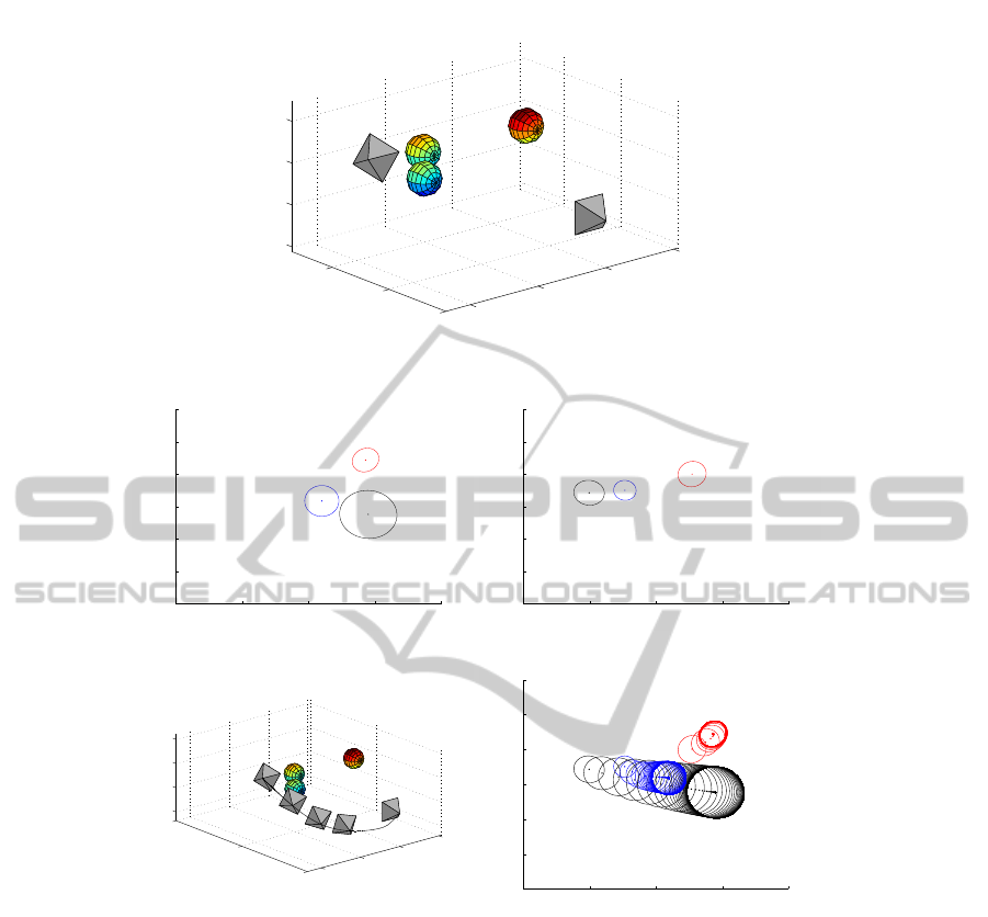
timation method, where the target consists of three
separate spheres as depicted in Fig. (3) (a). Radii and
positions of these spheres are supposed to be known.
Fig. (3) (b)-(c) are two views of the target obtained
at different camera poses F
o
and F
∗
. Relative camera
pose between F
∗
and F
o
is estimated using a virtual
VS method with Fig. (3) (d) showing the virtual cam-
era path generated by iteration (10)-(13) and Fig. (3)
(e) displaying the associated image trajectories. It is
noticed that there are two spheres occluded with each
other in the virtual servoing process, the situation of
which will fails a real VS task. Therefore, occlusion
among these spheres must be prevented by a path-
planning method, and it is also expected at the same
time that all of these spheres are kept in the field-of-
view of the camera. When an obstacle blocks the way
of the camera, collision between them is intended to
be avoided while satisfying simultaneously the other
constraints.
ICINCO2012-9thInternationalConferenceonInformaticsinControl,AutomationandRobotics
24
−20
−10
0
10
0
10
20
−5
0
5
10
F
*
x [mm]
z [mm]
F
o
y [mm]
(a)
0 200 400 600 800
0
100
200
300
400
500
600
(b)
0 200 400 600 800
0
100
200
300
400
500
600
(c)
−20
−10
0
10
0
20
40
−5
0
5
10
F
*
x [mm]
z [mm]
F
o
y [mm]
(d)
0 200 400 600 800
0
100
200
300
400
500
600
(e)
Figure 3: Pose estimation with three spheres. (a) Scenario. (b) Camera view in F
o
. (c) Camera view in F
∗
. (d) Virtual camera
path. (e) Virtual image trajectories.
3.2 Constraints
For all the above mentioned constraints, priority will
be given to the depth of the target, which is required to
be positive all the way along the camera path. Second,
collision in workspace will be prevented by adjusting
mainly the trajectories of camera translation. Third,
field-of-view limit is going to be met by restraining
projection of the target within the image size. When
the target consists of two or more separate entities,
occlusion among these entities will be prevented to
achieve visibility of all of them in the course of a real
VS process.
To describe the camera path with boundaries on
both sides, we use a path parameter w ∈ [0,1] with its
value 0 implying the start of the path F
o
, and value 1
meaning the end of the path F
∗
. Transition from F
o
to F
∗
is developed from the results in Section 3.1 and
denoted as {R,t} . Thus we have:
{R(0),t(0)} = {I
3×3
,0
3
},
{R(1),t(1)} = {R, t}.
(14)
Between the abovetwo camera poses, camera path
{R(w),t(w)} is intended to satisfy the following con-
straints.
3.2.1 Field-of-View
In arbitrary camera frame along the path, the target is
expected to be in the field-of-view of the camera. For
VisualServoingPath-planningwithSpheres
25
a point H mentioned in Section 2.1, its field-of-view
limit in camera frame {R(w),t(w)} is expressed as:
e
⊤
3
KR(w)
⊤
(H−t(w)) > 0,
0 < e
⊤
1
KR(w)
⊤
(H−t(w)) < ζ
x
,
0 < e
⊤
2
KR(w)
⊤
(H−t(w)) < ζ
y
,
(15)
where ζ
x
, ζ
y
are, respectively, the length and height of
an image in pixels.
For a sphere, depth of the sphere center is meant to
be larger than the sphere radius. In addition, extreme
values of the projection of the sphere that is drawn in
Fig. 2 are restricted to being located within the image
size:
z
o
−r > 0,
X
max
< ζ
x
,
Y
max
< ζ
y
,
X
min
,Y
min
> 0,
(16)
where X
max
, Y
max
, X
min
and Y
min
are computed from
image moments of the sphere:
X
max
=
¯
X +
√
µ
20
=
f(x
o
z
o
+ r
p
x
2
o
+ z
2
o
−r
2
)
z
2
o
−r
2
+
ζ
x
2
,
X
min
=
¯
X −
√
µ
20
=
f(x
o
z
o
−r
p
x
2
o
+ z
2
o
−r
2
)
z
2
o
−r
2
+
ζ
x
2
,
Y
max
=
¯
Y +
√
µ
02
=
f(y
o
z
o
+ r
p
y
2
o
+ z
2
o
−r
2
)
z
2
o
−r
2
+
ζ
y
2
,
Y
min
=
¯
Y −
√
µ
02
=
f(y
o
z
o
−r
p
y
2
o
+ z
2
o
−r
2
)
z
2
o
−r
2
+
ζ
y
2
.
(17)
Bring (17) into (16), we obtain a lot of inequalities in
the function of the sphere center:
ζ
x
2f
(z
2
o
−r
2
) −x
o
z
o
2
−r
2
(x
2
o
+ z
2
o
−r
2
) > 0,
ζ
x
2f
(z
2
o
−r
2
) −x
o
z
o
> 0,
ζ
x
2f
(z
2
o
−r
2
) + x
o
z
o
2
−r
2
(x
2
o
+ z
2
o
−r
2
) > 0,
ζ
x
2f
(z
2
o
−r
2
) + x
o
z
o
> 0,
ζ
y
2f
(z
2
o
−r
2
) −y
o
z
o
2
−r
2
(y
2
o
+ z
2
o
−r
2
) > 0,
ζ
y
2f
(z
2
o
−r
2
) −y
o
z
o
> 0,
ζ
y
2f
(z
2
o
−r
2
) + y
o
z
o
2
−r
2
(y
2
o
+ z
2
o
−r
2
) > 0,
ζ
y
2f
(z
2
o
−r
2
) + y
o
z
o
> 0.
(18)
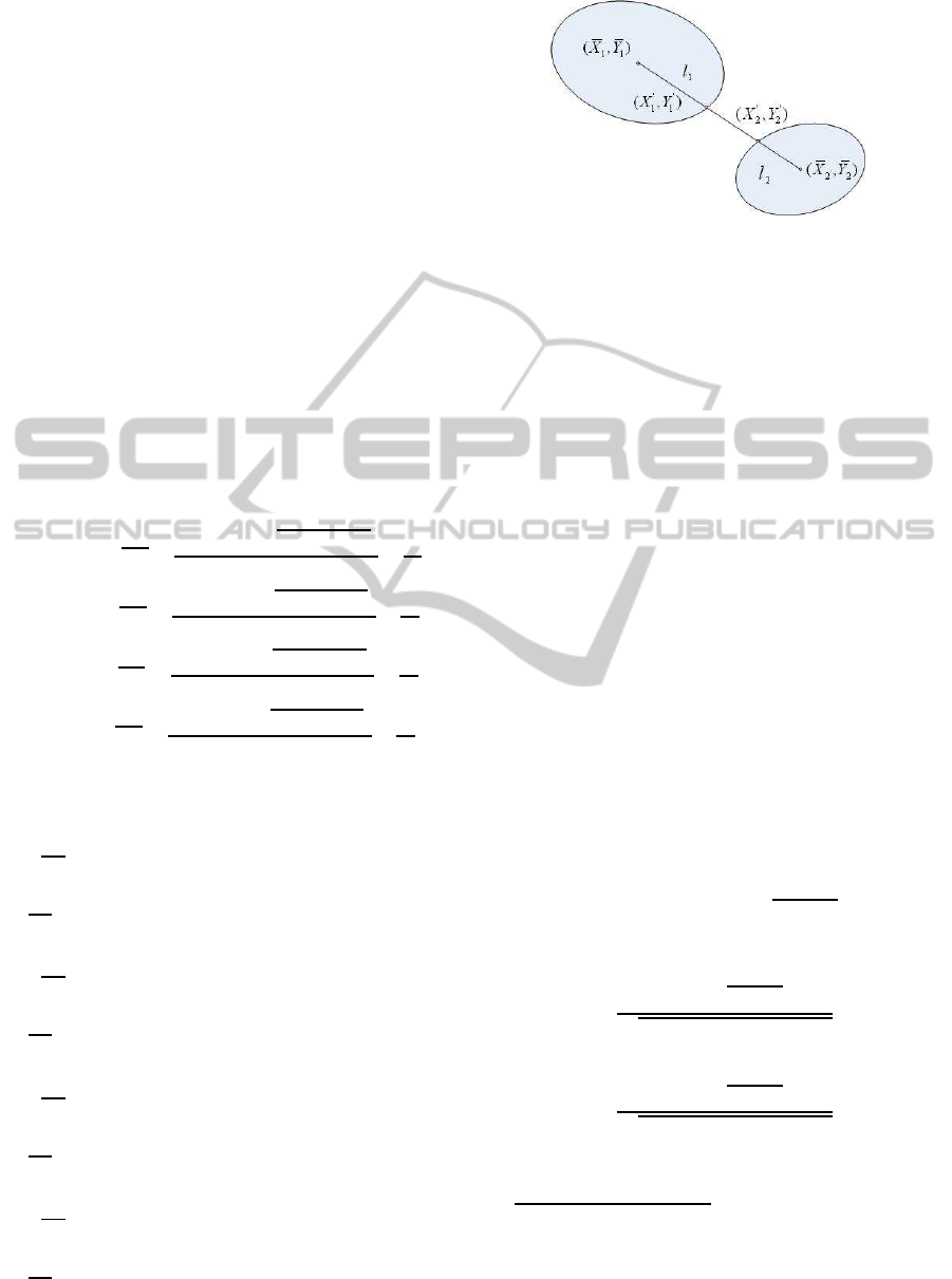
Figure 4: Projections of two spheres on the image plane.
Coordinates of the sphere center o = [x
o
,y
o
,z
o
]
⊤
in the above function are dependent on the camera
path {R(w),t(w)}, w ∈[0,1].
3.2.2 Occlusion
Two or more entities are demanded for constituting
a target in visual servoing with spheres. Occlusion
among these entities is expected to be avoided to
maintain the visibility of all of them. We take one
sphere and a point for example, the point will not hide
behind the sphere from the camera view by enforcing
the following restriction in workspace:
(H−o)
⊤
(t(w) −o) > 0, (19)
where H and o are respectively the coordinates of a
point and the sphere center expressed in the current
camera frame. This inequality guarantees that the
camera is above a plane that is perpendicular to the
vector (H−o) and passes through the sphere center.
When two spheres are included in one target, we
denote (
¯
X
1
,
¯
Y
1
) and (
¯
X
2
,
¯
Y
2
) the pixel coordinates of
two centers of their projections on the image plane, as
shown in Fig. 4. Line that passes through these two
ellipse centers is described as:
Y = (X −
¯
X
1
)α+
¯
Y
1
, α =
¯
Y
2
−
¯
Y
1
¯
X
2
−
¯
X
1
. (20)
We solve equation (3) and (20) together and then
calculate distance between (
¯
X
1
,
¯
Y
1
) and (
¯
X
′
1
,
¯
Y
′
1
) as
l
1
=
A
1
B
1
√
α
2
+ 1
p
µ
02
1
+ α
2
µ
20
1
−2αµ
11
1
, (21)
and distance between (
¯
X
2
,
¯
Y
2
) and (
¯
X
′
2
,
¯
Y
′
2
) as
l
2
=
A
2
B
2
√
α
2
+ 1
p
µ
02
2
+ α
2
µ
20
2
−2αµ
11
2
. (22)
As a result, occlusion between these two spheres
will be avoided by imposing the following inequality:
q
(
¯
X
1
−
¯
X
2
)
2
+ (
¯
Y
1
−
¯
Y
2
)
2
−l
1
(α) −l
2
(α) > 0. (23)
Three similar inequalities will be used to avoid
self-occlusion of the target when it consists of three
spheres.
ICINCO2012-9thInternationalConferenceonInformaticsinControl,AutomationandRobotics
26

3.2.3 Collision
Let b ∈ R
3
be an obstacle in workspace expressed
in the reference frame F
o
. Coordinates of this obsta-
cle in the current camera frame is R(w)
⊤
(b−t(w)).
Collision between the current camera frame and the
obstacle is avoid by defining a tolerance distance d:
kR(w)
⊤
(b−t(w))k
2
−d
2
> 0. (24)
3.3 Polynomial Parametrization
We use polynomials in path parameter w to model tra-
jectories of camera translation and rotation:
(
q(w) = U·[w
σ
,..., w,1]
⊤
,
t(w) = V·[w
τ
,..., w,1]
⊤
,
(25)
where q(w) is Cayley representation (Craig, 2005) of
the rotation matrix:
[q(w)]
×
= (R(w) −I
3×3
)(R(w) + I
3×3
)
−1
. (26)
Boundaries defined in (14) will be satisfied by as-
signing the first and last columns in the coefficient
matrices in (25) with the following values and letting
the middle of these matrices, that is
˜
U ∈ R
3×(σ−1
)
and
˜
V ∈ R
3×(τ−1
), to be variable:
(
U =
q(1) −
˜
U·1
σ−1
,
˜
U,0
3
,
V =
t(1) −
˜
V·1
τ−1
,
˜
V,0
3
.
(27)
Matrices
˜
U and
˜
V will be assigned a ”guess” value
and substituted in (25) and then (16), (23) and (19) to
calculate the left hand side of all the inequalities for
all the entities and all the way along the path with
w ∈ (0,1). A minimum value of the left hand side of
all the inequalities will be obtained. If this minimum
value is negative, nonlinear optimization will be used
to search for appropriate values for
˜
U and
˜
V until the
minimum of all the calculation is positive. Till this
end, all the constraints will be satisfied.
Planned image trajectories will be generated by
bringing new values of
˜
U and
˜
V into (25), (3) and
(4). These trajectories will be followed by an IBVS
controller (Mezouar and Chaumette, 2002a):
T
c
= −λ
1
ˆ
L
+
(s(t) −s
p
(w)) +
ˆ
L
+
ds
p
(w)
dt
, (28)
where the feature set is determined as specified in
Section 3.1 with s(t) holding the current values and
s
p
(w) being the planned ones when w = 1 −e
−tλ
2
.
Interaction matrix or image jacobian (Mezouar and
Chaumette, 2002b) regarding the features of a sphere
is a stack of matrices L
s
12
and L
s
3
. Matrix L
s
12
corre-
sponds to the centroid of the projection of the sphere:
L
s
12
=
−1/¯z 0
0 −1/¯z
¯
X/¯z+ aµ
20
+ bµ
11
¯
Y/¯z+ aµ
11
+ bµ
02
¯
X
¯
Y + µ
11
1+
¯
Y
2
+ µ
02
−1−
¯
X
2
−µ
20
−
¯
X
¯
Y −µ
11
¯
Y −
¯
X
⊤
,
where ¯z is not the depth of the sphere center, and
¯z =
1
a
¯
X + b
¯
Y + c
= z
o
−r
2
/z
o
,
a = x
o
/(x
2
o
+ y
2
o
+ z
2
o
−r
2
),
b = y
o
/(x
2
o
+ y
2
o
+ z
2
o
−r
2
),
c = z
o
/(x
2
o
+ y
2
o
+ z
2
o
−r
2
),
(29)
while L
s
3
corresponds to the half of the sum of µ
02
and µ
20
:
L
s
3
=
−aµ
20
−bµ
11
−aµ
11
−bµ
02
(
1
¯z
+ a
¯
X)µ
20
+ (
1
¯z
+ b
¯
Y)µ
02
+ µ
11
(b
¯
X +a
¯
Y)
2
¯
Yµ
02
+
¯
Xµ
11
+
¯
Yµ
20
−2
¯
Xµ
20
−
¯
Yµ
11
−
¯
Xµ
02
0
⊤
.
The second addend in (28) is a compensation item
provided by the derivation of e =
ˆ
L
+
(s(t) −s
p
(w))
(Mezouar and Chaumette, 2002a), and in this paper
we have:
ds
p
(w)
dt
=
ds
p
(w)
dw
·
dw
dt
= λ
2
e
−tλ
2
ds
p
(w)
dw
.
For features selected for a sphere, their derivatives
with respect to the path parameter w are listed:
d
¯
X
dw
=
f
(z
2
o
−r
2
)
2
h
z
o
(z
2
o
−r
2
)
dx
o
dw
−x
o
(z
2
o
−r
2
)
dz
o
dw
i
,
d
¯
Y
dw
=
f
(z
2
o
−r
2
)
2
h
z
o
(z
2
o
−r
2
)
dy
o
dw
−y
o
(z
2
o
−r
2
)
dz
o
dw
i
,
dµ
02
dw
=
2f
2
r
2
(z
2
o
−r
2
)
3
h
y
o
(z
2
o
−r
2
)
dy
o
dw
−z
o
(2y
2
o
+ z
2
o
−r
2
)
dz
o
dw
i
,
dµ
20
dw
=
2f
2
r
2
(z
2
o
−r
2
)
3
h
x
o
(z
2
o
−r
2
)
dx
o
dw
−z
o
(2x
2
o
+ z
2
o
−r
2
)
dz
o
dw
i
,
d
dw
(
µ
20
+ µ
02
2
) =
1
2
dµ
02
dw
+
dµ
20
dw
.
4 EXAMPLES
Synthetic scene is generated using MATLAB to verify
the proposed scheme. The first example aims to avoid
collision in the Cartesian space while keeping visible
all the entities that consist of a target. The second
example gives a planned path that prevents occlusion
VisualServoingPath-planningwithSpheres
27
−20
−10
0
10
0
20
40
−5
0
5
10
F
*
x [mm]
z [mm]
F
o
y [mm]
(a)
0 200 400 600 800
0
100
200
300
400
500
600
(b)
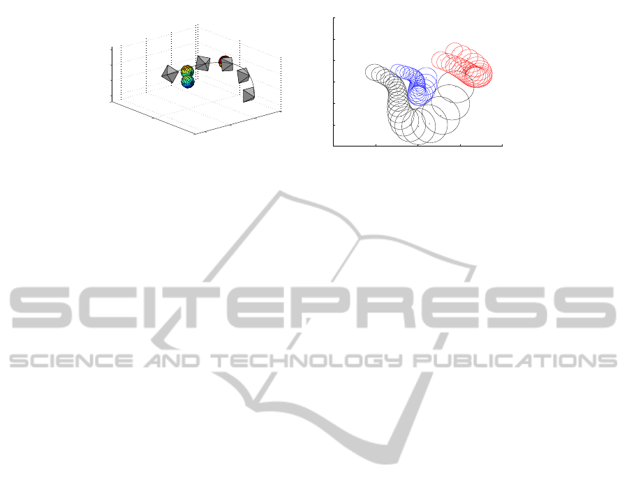
Figure 5: Occlusion avoidance among three spheres. (a) Camera path. (b) Image trajectories.
among three spheres and simultaneously meets field-
of-view limit for all of them. Whatever the selected
features are in an image of size 800 ×600 pixels,
normally distributed image noises range from (−1,1)
pixels are added upon them.
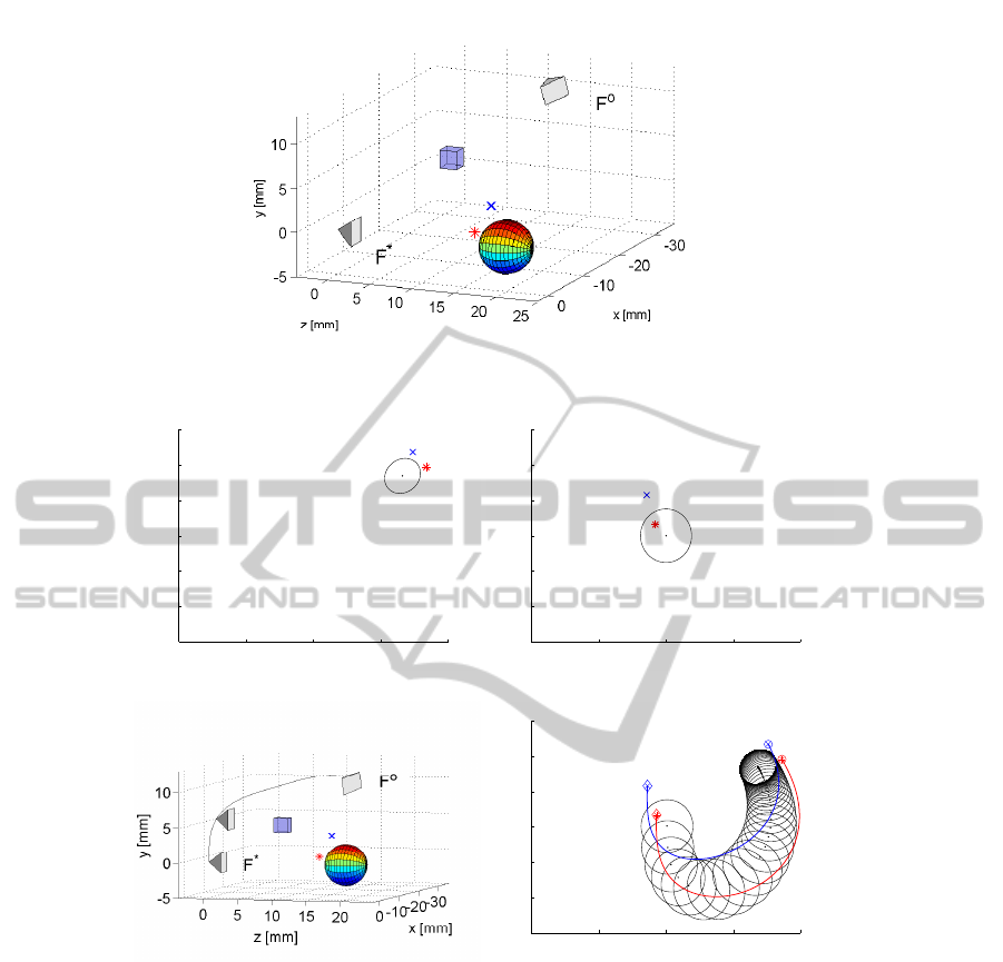
4.1 Collision Avoidance
In this example, the target consist of a sphere and
two points. As depicted in Fig. 6 (a), the sphere
has radius of 3 mm and its center coordinates as
[0,0,20]
⊤
mm expressed in F
∗
. The other two points
are symbolized respectively as a star and an x-mark
beside the sphere. An obstacle represented by a
box is found between the two camera poses F
∗
=
{I
3×3
,0
3
} and F
o
= {e
[ρ]
×
,[−35,10,10]
⊤
mm} with
ρ = [π/12,π/4,−π/6]. Intrinsic parameters of the
camera are estimated as follows:
K =
508 0 403
0 496 302
0 0 1
. (30)
Camera views of the target obtained in F
o
and F
∗
are separately displayed in Fig. 6 (b) and (c). Fea-
tures extracted from these camera views are pixel co-
ordinates of the centroid of the ellipse, that is
¯
X and
¯
Y, combination of the length of the major and mi-
nor semi-axes of the ellipse, that is (A
2
+ B
2
)/2, and
pixel coordinates of image projections of the other
two points. This is exactly the same as the feature
set mentioned in (8). Given the position and model
of the target, relative camera pose between F
∗
and F
o
is estimated using a virtual VS method and is used
as boundaries for the planned camera path. Fig. 6
(d) plots the satisfactory camera path that avoids col-
lision with a given obstacle and keeps the sphere and
also the other two points in the field-of-view of the
camera. It is also noticed that the two other points
are not occluded by the sphere along the camera path
by applying constraints as shown in (19). Fig. 6 (e)
demonstrates visibility of all the entities that consist
of the target in this example, where circles are used to
imply the start of image trajectories of the points and
diamonds the end of them.
4.2 Occlusion Avoidance
The scenario for visual servoing path-planning with
three spheres is illustrated in Fig. 3 (a), where these
three spheres have the same radius of 2 mm and po-
sitions of their centers as [−10,2,20]
⊤
, [−6,3,25]
⊤
and [5, 5,20]
⊤
expressed in F
∗
. Occlusion avoidance
among these spheres and the maintenance of camera
view of them are expected to be achieved during a real
time VS. Boundaries of this camera path are demon-
strated in Fig. 3 (a) as F
∗
= {I
3×3
,0
3
} and F
o
=
{e
[ρ]
×
,[−20,7,18]
⊤
mm}with ρ = [0,π/3,−π/6]. In-
trinsic parameters of the camera are approximated as:
K =
410 0 405
0 380 305
0 0 1
.
Relative camera pose between F
∗
and F
o
is esti-
mated using a virtual VS method based on the feature
set stated in (9). This feature set is a stack of
¯
X,
¯
Y and
(A
2
+B
2
)/2 for each sphere and can be extracted from
the projection of the sphere in F
o
and F
∗
as shown in
Fig. 3 (b)-(c). The corresponding virtual camera path
and image trajectories are also displayed separately in
Fig. 3 (d) and (e). It is obvious that in Fig. 3 (e) there
are two spheres occluded with each other, the case of
which will fail a real VS task. Therefore, the pro-
posed path-planning approach is intended to generate
another camera path meeting the required constraints
in this example. The resulting camera path and image
trajectories are shown in Fig. 5 (a)-(b), where occlu-
sions are perfectly avoided with trajectories of all the
spheres kept in the field-of-view of the camera.
ICINCO2012-9thInternationalConferenceonInformaticsinControl,AutomationandRobotics
28
(a)
0 200 400 600 800
0
100
200
300
400
500
600
(b)
0 200 400 600 800
0
100
200
300
400
500
600
(c)
(d)
0 200 400 600 800
0
100
200
300
400
500
600
(e)
Figure 6: Collision avoidance in workspace. (a) Scenario (b) Camera view in F
o
. (c) Camera view in F
∗
. (d) Camera path.
(e) Image trajectories.
5 CONCLUSIONS
This paper proposes a path-planning approach for vi-
sual servoing with spheres. Sphere is a very special
object that projects in the image plane as an ellipse
whose centroid may not correspond to the center of
the sphere. One sphere only provides three indepen-
dent features. Therefore, this paper combines a sphere
with at least two points or at least two other spheres
to serve as a target. In each of the two cases, cam-
era view of the whole target is obtained and also the
sphere is prevented occluding other entities in the tar-
get. Simulations validate the proposed path-planning
approach. Future work is meant to include constraints
in joint space. Also, path-planning from objects that
are more complicated than a sphere, such as a bottle,
are interesting to explore.
REFERENCES
Chaumette, F. (1998a). De la perception l’action :
l’asservissement visuel; de l’action la perception :
la vision active. PhD thesis, Universit de Rennes 1.
Chaumette, F. (1998b). Potential problems of stability and
convergence in image-based and position-based visual
VisualServoingPath-planningwithSpheres
29

servoing. In Kriegman, D., Hager, G., and Morse, S.,
editors, The Confluence of Vision and Control, pages
66–78. vol. 237 of Lecture Notes in Control and Infor-
mation Sciences, Springer-Verlag.
Chaumette, F. (2004). Image moments: a general and useful
set of features for visual servoing. IEEE Trans. on
Robotics, 20(4):713–723.
Chaumette, F. and Hutchinson, S. (2006). Visual servo con-
trol, part I: Basic approaches. IEEE Robotics and Au-
tomation Magazine, 13(4):82–90.
Chaumette, F. and Hutchinson, S. (2007). Visual servo con-
trol, part II: Advanced approaches. IEEE Robotics and
Automation Magazine, 14(1):109–118.
Chesi, G. (2009). Visual servoing path-planning via homo-
geneous forms and lmi optimizations. IEEE Trans. on
Robotics, 25(2):281–291.
Chesi, G. and Hashimoto, K., editors (2010). Visual Servo-
ing via Advanced Numerical Methods. Springer.
Chesi, G., Hashimoto, K., Prattichizzo, D., and Vicino, A.
(2004). Keeping features in the field of view in eye-
in-hand visual servoing: A switching approach. IEEE
Trans. on Robotics, 20(5):908–914.
Chesi, G. and Hung, Y. S. (2007). Global path-planning for
constrained and optimal visual servoing. IEEE Trans.
on Robotics, 23(5):1050–1060.
Chesi, G. and Vicino, A. (2004). Visual servoing for
large camera displacements. IEEE Trans. on Robotics,
20(4):724–735.
Collewet, C. and Marchand, E. (2010). Luminance: A
new visual feature for visual servoing. In Chesi, G.
and Hashimotos, K., editors, Visual Servoing via Ad-
vanced Numerical Methods, pages 71–90. vol. 401 of
Lecture Notes in Control and Information Sciences,
Springer-Verlag.
Cowan, N., Weingarten, J., and Koditschek, D. (2002). Vi-
sual servoing via navigation functions. IEEE Trans.
on Robotics and Automation., 18(4):521–533.
Craig, J., editor (2005). Introduction to Robotics: Mechan-
ics and Control. Pearson Education.
Gans, N. and Hutchinson, S. (2007). Stable visual servoing
through hybrid switched-system control. IEEE Trans.
on Robotics, 23(3):530–540.
Hashimoto, K., Kimoto, T., Ebine, T., and Kimura, H.
(1991). Manipulator control with image-based visual
servo. In Proc. IEEE Int. Conf. Robot. Automat., pages
2267–2272, San Francisco, CA.
Malis, E., Chaumette, F., and Boudet, S. (1999). 2 1/2 d vi-
sual servoing. IEEE Trans. on Robotics and Automa-
tion, 15(2):238–250.
Mezouar, Y. and Chaumette, F. (2002a). Path planning for
robust image-based control. IEEE Trans. on Robotics
and Automation, 18(4):534–549.
Mezouar, Y. and Chaumette, F. (2002b). Path planning for
robust image-based control. IEEE Trans. on Robotics
and Automation., 18(4):534–549.
Oh, P. Y. and Allen, P. K. (2001). Visual servoing by parti-
tioning degrees of freedom. IEEE Trans. on Robotics
and Automation, 17(1):1–17.
Shen, T. and Chesi, G. (2012). Visual servoing path-
planning for cameras obeying the unified model. Ad-
vanced Robotics, 26(8–9):843–860.
Tahri, O. and Chaumette, F. (2005). Point-based and region-
based image moments for visual servoing of planar
objects. IEEE Trans. on Robotics, 21(6):1116–1127.
Tahri, O., Mezouar, Y., Chaumette, F., and Araujo, H.
(2010). Visual servoing and pose estimation with
cameras obeying the unified model. In Chesi, G.
and Hashimotos, K., editors, Visual Servoing via Ad-
vanced Numerical Methods, pages 231–252. vol. 401
of Lecture Notes in Control and Information Sciences,
Springer-Verlag.
Tatsambon Fomena, R. and Chaumette, F. (2008). Visual
servoing from two special compounds of features us-
ing a spherical projection model. In IEEE/RSJ Int.
Conf. on Intelligent Robots and Systems, IROS’08,
pages 3040–3045, Nice, France.
Taylor, C. and Ostrowski, J. (2000). Robust vision-based
pose control. In IEEE Int. Conf. Robot. Automat.,
pages 2734–2740, San Francisco, CA.
ICINCO2012-9thInternationalConferenceonInformaticsinControl,AutomationandRobotics
30
