
Data-based Tuning of PI Controllers for Vertical Three-Tank Systems
Mircea-Bogdan Rădac
1
, Bogdan-Alexandru Bigher
1
, Radu-Emil Precup
1
, Emil M. Petriu
2
,
Claudia-Adina Dragoş
1
, Stefan Preitl
1
and Alexandra-Iulia Stînean
1
1
Dept. of Automation and Appl. Inf., “Politehnica” University of Timisoara, Bd. V. Parvan 2, 300223 Timisoara, Romania
2
School of Electrical Eng. and Computer Science, University of Ottawa, 800 King Edward, Ottawa, ON, K1N 6N5, Canada
Keywords: Iterative Feedback Tuning, Level Control, PI Controllers, Vertical Three-tank Systems.
Abstract: This paper suggests the application of Iterative Feedback Tuning (IFT) as a data-based control technique to
parameter tuning of PI controllers dedicated to vertical three-tank systems. The level control in the first two
tanks is carried out using a multivariable control system structure which consists of two control loops, one
for each level. The two PI controllers in these control loops are first tuned in terms of the Modulus
Optimum method. New IFT algorithms are proposed in order to ensure the performance improvement of
level control systems by means of six steps assisted by experiments. The experimental results show the
strong performance improvement obtained after few iterations of IFT algorithms in terms of a model
reference tracking optimization problem.
1 INTRODUCTION
Vertical three-tank systems are nonlinear Multi
Input-Multi Output (MIMO) benchmarks which
convincingly illustrate control design, fault detection
and diagnosis problems. Some current approaches to
the level control of vertical three-tank systems
include fault diagnosis using sliding mode observers
(Orani et al., 2010), fuzzy model-based predictive
control (Ahmed et al., 2010), discrete-time model
identification (Nikolić et al., 2010), sensitivity
analysis of process models (Antić et al., 2011) and
optimal tuning of PID controllers by nature-inspired
algorithms (Kumar and Dhiman, 2011).
The improvement of control system performance
indices (settling time, overshoot, etc.) for these
nonlinear MIMO processes can be carried out by
data-based tuning in terms of experiment-based
solving of optimization problems. Iterative Feedback
Tuning (IFT) (Hjalmarsson et al., 1994, 1998);
(Hjalmarsson, 2002) is a popular data-based control
technique which makes use of the input-output data
measured from the closed-loop system during its
operation to calculate the estimates of the gradients
and eventually Hessians of the objective functions.
Several experiments are conducted per iteration and
the updated controller parameters are obtained on
the basis of input-output data and estimates.
The efficiency of IFT applied to MIMO
processes is proved in several applications
(Hjalmarsson, 1998); (Sjöberg et al., 2003);
(Huusom et al., 2009); (Rădac et al., 2009);
(McDaid et al., 2010); (Precup et al., 2010); (Precup
et al., 2012). This paper is built upon the IFT
algorithms applied to tuning of PID controllers and
PI-fuzzy controllers in level control problems for
horizontal three-tank systems (Precup et al., 2010);
(Precup et al., 2012). MIMO control systems which
consist of two control loops for each level control
are involved. The main contribution of this paper is
represented by new IFT algorithms which ensure the
performance improvement of PI control systems
dedicated to the first two tanks. The two PI
controllers are first tuned using simple process in
terms of the Modulus Optimum (MO) method
referred by Åström and Hägglund (1995). The six
steps of the IFT algorithms are next applied making
use of a unified formulation.
Our approach offers twofold advantages with
respect to the state-of-the-art. First, a cost-effective
systematic tuning approach for nonlinear MIMO
processes is offered. Second, the experimental
validation is carried out.
This paper is structured as follows. The problem
setting concerning IFT applied to level control of
vertical three-tank systems is presented in the next
section. The nonlinear process models and the
31
R
ˇ
adac M., Bigher B., Precup R., Petriu E., Drago¸s C., Preitl S. and Stînean A..
Data-based Tuning of PI Controllers for Vertical Three-Tank Systems.
DOI: 10.5220/0003998500310039
In Proceedings of the 9th International Conference on Informatics in Control, Automation and Robotics (ICINCO-2012), pages 31-39
ISBN: 978-989-8565-21-1
Copyright
c
2012 SCITEPRESS (Science and Technology Publications, Lda.)

simplified process models used in the initial
controller tuning are given in Section 3. The new
IFT algorithms are presented in Section 4. The
experimental results offered in Section 5
convincingly show the performance improvement.
The conclusions are highlighted in Section 6.
2 PROBLEM SETTING
The process in vertical three-tank systems (Figure 1,
derived from (Inteco, 2007)) consists of three tanks
of different shapes located vertically (T1, T2 and
T3), a fourth reflux tank (T4) placed under the lower
tank, a variable speed pump driven by a DC motor
that supplies the upper tank T1, and three electrical
servo valves (SV1, SV2 and SV3) which determine
the outflow from each tank. The three tanks are
equipped with piezo-resistive pressure sensors PS1,
PS2 and PS3 which measure the water levels H
1
, H
2
and H
3
, respectively.
Figure 1: Structure of controlled process in vertical three-
tank systems viewed as multi-tank systems according to
(Inteco, 2007).
Several Single Input-Single Output (SISO) and
MIMO control system structures can be considered
as shown by Bigher (2011) on the basis of Figure 1
using different combinations of the four inputs q –
the inflow to T1, C
1
– the resistance of the output
orifice of T1, C
2
– the resistance of the output orifice
of T2, and C
3
– the resistance of the output orifice of
T3. This paper considers the MIMO control system
dedicated to the levels H
1
and H
2
and organized in
terms of Figure 2.
The typical control objectives concerning the
control system structure presented in Figure 2 are to
keep the desired liquid levels in the tanks T1 and T2,
viz. H
1
and H
2
, as specified by the two reference
inputs r
1
and r
2
, respectively, which belong to the
reference input vector
T
rr ][
21
=r
(T stands for
matrix transposition) and carry out the rejection of
two possible disturbances (gathered in the
disturbance input vector d) represented by C
2
and/or
C
3
. These disturbances usually model sudden
demands of water from the downstream water
distribution networks. The control system structure
given in Figure 2 assumes that the level in the tank
T3, H
3
, is a response which is uncontrollable, and
that the pressure sensors PS1, PS2 and PS3 are
included in the process dynamics (P).
Figure 2: Structure of MIMO control system.
As suggested by Precup et al. (2010), a simple
control system structure that can fulfil these control
objectives is presented in Figure 3. Figure 3 points
out a MIMO control system structure with two
control loops dedicated to the separate control of H
1
and H
2
, where,
111
Hre −=
and
222
Hre −=
are the
control errors, C
1
(s) and C
2
(s) are the SISO
controllers which build the MIMO controller
emphasized in Figure 2, and the two control signals
(in relation with Figure 2) are:
121
, Cuqu ==
.
(1)
Figure 3: Structure of two control loops in MIMO control
system.
The separate control of H
1
and H
2
by means of
the control system structure presented in Figure 3 is
justified as:
ICINCO2012-9thInternationalConferenceonInformaticsinControl,AutomationandRobotics
32

There is no need for decoupling controllers
because it is considered that the two channels (which
correspond to H
1
and H
2
) represent additional
disturbances and included in d. Controllers with
integral components solve the disturbance rejection
and thus the decoupling.
It is very convenient to design and tune
separately the controllers with the transfer functions
C
1
(s) and C
2
(s).
IFT will be used in the sequel to tune the parameters
of the controllers with the transfer functions C
1
(s)
and C
2
(s) by two IFT algorithms. Accepting, for
simplicity, the control system structure for one of the
two controllers, the structure of this IFT-based
control system is illustrated in Figure 4, where: r –
the reference input (r
1
or r
2
), d – the disturbance
input (an element of d), e – the control error (e
1
or
e
2
), u – the control signal (u
1
or u
2
), ρ – the
parameter vector containing the controller
parameters, C(ρ) – the controller transfer function
(C
1
(s) or C
2
(s), and the argument s is omitted to
simplify the presentation), F – the reference model
transfer function, P – the process transfer function, y
– the controlled output (H
1
or H
2
), y
d
– the desired
output (of reference model), and
d
yyy −=δ
– the
tracking error.
Figure 4: IFT-based control system structure for one
control loop.
The model reference tracking optimization
problem, numerically solved in an experiment-based
iterative way by IFT algorithms, is defined as
)(minarg
*
ρρ
ρ
J
D∈ρ
=
,
(2)
where
)(ρJ
is the objective function:
2
1
)],([)/5.0()( ρρ kyNJ
N
k
δ=
∑
=
,
(3)
N is the number of samples, i.e., the length of an
experiment conducted in the framework of IFT
algorithms,
*
ρ
is the optimal parameter vector
produced by IFT algorithms, and
ρ
D
is the feasible
domain for
ρ which accounts for several constraints
including stability ones (Hjalmarsson, 2002);
(Sjöberg et al., 2003); (Huusom et al., 2009); (Rădac
et al., 2011).
3 PROCESS MODELS
The mass-balance equations lead to the following
first principle state-space equations of the process
(Inteco, 2007):
1
112
3
2
1111111
21122 22 22
32233 3333
/() /(),
/() /(),
/() /(),
Hq H CH H
HCH H CH H
HCH H CH H
α
αα
α
α
ββ
ββ
ββ
=−
=−
=−
&
&
&
(4)
where
l
α
,
}3,2,1{∈l
, is the flow coefficient of
th
i
tank, and
)(
ll
H
β
,
}3,2,1{∈l
, is the cross sectional
area of
th
i
tank at the level
i
H
:
11 2 2 2 2max
22
33 3
() , () / ,
() ( ),
Haw HcwHH
HRRH
ββ
β
==+
=−−
(5)
and the geometrical parameters in (5) depend on the
shapes of the three tanks (Inteco, 2007).
Since the nonlinear state-space equations (4) are
complicated to use in the design, the least-squares
identification is applied to obtain the parameters of
the following transfer functions of the simplified
models which correspond to the processes in the two
control loops in Figure 3 (Bigher, 2011):
, ),1)(1/[(
)(/)()(
, ),1)(1/[(
)(/)()(
22222
122
11111
11
TTsTsTk
sCsHsP
TTsTsTk
sqsHsP
P
P
<<++=
=
<<++=
=
ΣΣ
ΣΣ
(6)
where:
21
,
PP
kk
– the process gains,
21
,
ΣΣ
TT
– the
small time constants, and
21
,TT
– the large time
constants. As shown in (Åström and Hägglund,
1995), PI controllers can offer good control system
performance indices for processes characterized by
the transfer functions
)(
1
sP
and
)(
2
sP
. The transfer
functions of the two continuous-time PI controllers
are:
ssTksC
jcjcj
/)1()(
+=
,
}2,1{∈j
,
(7)
where
jc
k
is the controller gain and
jc
T
is the
integral time constant,
}2,1{∈j
.
The performance of the two control system with
Data-basedTuningofPIControllersforVerticalThree-TankSystems
33

these two PI controllers is improved by two IFT
algorithms presented in the next section. The
improvement involves the iterative data-based
solving of the optimization problem (2).
4 IFT ALGORITHMS
The two IFT algorithms applied to tune the
parameters of the two PI controllers in the control
system structure given in Figure 3 are expressed in
terms of the following unified steps, with the steps 2
to 6 repeated at each iteration:
Step 1. The MO method is applied to tune the
parameters of the initial PI controllers with the
transfer functions given in (7). The tuning equations
of the two PI controllers are:
, ),2/(1
jjcjjPjc
TTTkk ==
Σ
}2,1{∈j
.
(8)
The sampling period
s
T
is set and the continuous-
time PI controllers are discretized to obtain the
transfer functions of the two discrete-time PI
controllers:
},2,1{
),1/()()(
11
2 1
1
∈
−ρ+ρ=
−−−
j
zzzC
i
j
i
jj
(9)
where the superscript i stands for the iteration index,
0=i
at step 1, and the parameter vectors of the two
controllers are
}2,1{ ,][
2 1
∈ρρ= j
Ti
j
i
j
i
ρ
.
(10)
The reference models for the two control loops are
obtained by discretizing the continuous-time
reference model with the transfer function
)2/()(
2
00
22
0
ω+ςω+ω= sssF
,
(11)
where the damping ratio
ς
and the natural resonant
frequency
0
ω
are set such that to fulfil the
performance specifications imposed to the MIMO
control system.
Step 2. A first experiment, referred to as the
normal experiment, is conducted with the reference
input vector
r applied to the control system, and the
controlled outputs
)(
1
i
y ρ
are recorded for each
level. The tracking error is calculated as
)(),(),(
1
kykyky
d
ii
−=δ ρρ
, where the superscript
1 indicates this first experiment.
Step 3. A second experiment, referred to as the
gradient experiment, is conducted with the output
vector from the first experiment applied to the
control system as reference input, and the controlled
outputs
)(
2 i
y ρ
are recorded for each level, where
the superscript 2 indicates this second experiment.
Step 4. The estimate of the gradient of
yδ
is
calculated in terms of:
)],,(
),([
)(
)/(1
)],(),([
),(
),(
1
),(
2
1
1
2 1
1
1
2 1
21
1
1
i
i
i
j
i
j
i
j
i
j
iii
j
i
j
i
ky
ky
qq
q
kyky
q
C
qC
k
y
est
ρ
ρ
ρρρ
ρ
ρ
ρ
ρ
−
⎥
⎥
⎦
⎤
⎢
⎢
⎣
⎡
ρ+ρ
ρ+ρ
=
−
∂
∂
⋅
=
⎥
⎦
⎤
⎢
⎣
⎡
∂
δ∂
−−
−
−
−
(12)
where
1−
q
is the backward shift operator.
Step 5. The gradient of the objective function is
calculated using (12) and
.),(),()/1(
)(
1
∑
=
⎭
⎬
⎫
⎩
⎨
⎧
⎥
⎦
⎤
⎢
⎣
⎡
∂
δ∂
δ=
⎥
⎦
⎤
⎢
⎣
⎡
∂
∂
N
k
ii
i
k
y
estkyN
J
est
ρ
ρ
ρ
ρ
ρ
(13)
Step 6. The next set of parameters
1+i
ρ
is
calculated according to the update law
⎥
⎦
⎤
⎢
⎣
⎡
∂
∂
γ−=
−
+
)(
1
1 i
ii
ii
J
est ρ
ρ
Rρρ
,
(14)
where
0>
γ
i
is the step size, and the positive
definite regular matrix
R
i
is typically a Gauss-
Newton approximation of the Hessian of J or the
identity matrix in the simplest case. The identity
matrix corresponding to the steepest descent method
is set in these two IFT algorithms.
The IFT algorithms are stopped after observing a
sufficient decrease of the objective function. A
trade-off to the number of experiments and to the
performance improvement should be ensured.
The convergence of the IFT algorithms is
ensured if the following step sizes are employed
(Hjalmarsson, 2002; Huusom et al., 2009):
∑∑
∞
=
∞
=
∞<γ∞=γ
0
2
0
,
i
i
i
i
,
(15)
and a convenient choice for the step size sequence is
(Rădac et al., 2011):
10.5 ,1 , ,
0
≤α<≥∈
γ
=γ
α
ii
i
i
N
,
(16)
ICINCO2012-9thInternationalConferenceonInformaticsinControl,AutomationandRobotics
34

where the initial step size
0
0
>
γ
is set such that to
ensure a compromise to the numerical stability and
to the convergence speed. In the situation where the
noise affects the measurements, a third normal
experiment should be performed in order to obtain
an unbiased estimate of the gradient of the objective
function.
5 EXPERIMENTAL RESULTS
The two IFT algorithms expressed in the unified
given in the previous section are applied to tune the
parameters of the PI controllers of the INTECO
multi-tank system laboratory equipment (Inteco,
2007). The values of the parameters of the simplified
process models (6) are (Bigher, 2011):
83.0
1
=
P
k
,
5.0
2
=
P
k
,
s 2
1
=
Σ
T
,
s 5
2
=
Σ
T
,
s 50
21
== TT
. The
main results related to the application of the IFT
algorithms are presented as follows.
The reference model (11) with the parameters
9.0=
ς
and
1
0
s 2292.0
−
=ω
is set for the IFT
algorithm dedicated to H
1
, and
1=
ς
and
1
0
s 1719.0
−
=ω
for the IFT algorithm dedicated to
H
2
. The reference models are chosen to be similar to
the initial closed loop response in order to ensure the
convexity of the cost function (Bazanella et al.,
2008). Several intermediate reference models can be
chosen before arriving at the final design, known as
the windsurfing approach (Hjalmarsson 2002). The
step size sequence (16) with
1=α
and
100
0
=
γ
is
introduced in the update law (14) of the IFT
algorithm dedicated to H
1
, and
1=α
and
50
0
=
γ
for the IFT algorithm dedicated to H
2
. From the
application point of view, the typical IFT gradient
experimental setup in which the control error from
the normal experiment is injected as reference can
not be used here. Instead, the output from the normal
experiment is used as a reference input since it is
just a filtered version of the reference from the
normal experiment and therefore it brings the closed
loop in the vicinity of the original trajectory. This
setup is also possible because the closed-loop system
has no resonant modes which could amplify the
corresponding frequencies.
The application of MO tuning equations (8),
setting the sampling period
s 1=
s
T
and the
application of Tustin’s discretization method lead to
the following initial values of the parameters of the
discrete-time PI controllers:
.9.9 ,1.10
,85.14 ,15.15
0
2 2
0
2 1
0
1 2
0
1 1
−=ρ=ρ
−=ρ=ρ
(17)
The parameters of the discrete-time PI controllers
after nine iterations of the IFT algorithm dedicated
to H
1
and five iterations of the IFT algorithm
dedicated to H
2
are:
.8534.9 ,1489.10
,8256.14 ,1758.15
5
2 2
5
2 1
9
1 2
9
1 1
−=ρ=ρ
−=ρ=ρ
(18)
The evolution of the objective function
corresponding to H
1
is illustrated in Figure 5.
Figure 5: Objective function versus iteration number for
control loop controlling H
1
.
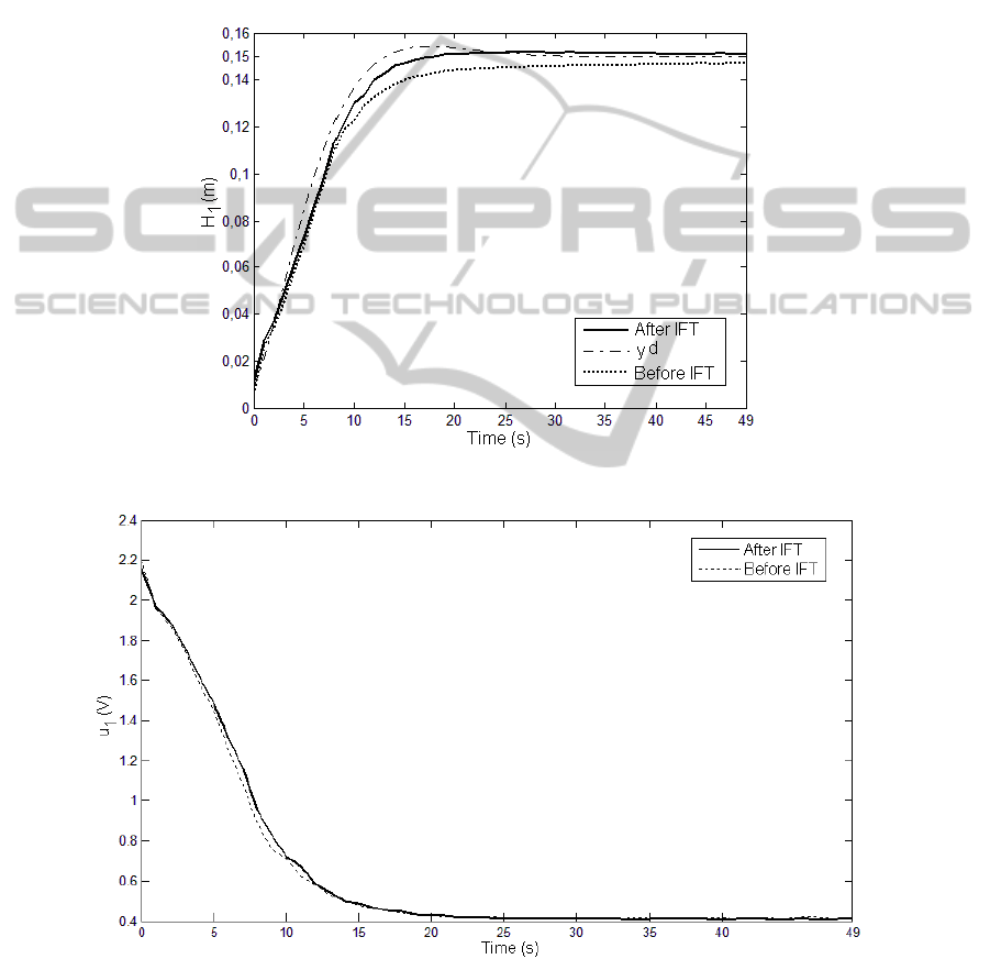
The experimental results concerning the behaviour
of the control loop for H
1
before and after the
application of the IFT algorithm are presented in
Figure 6 and in Figure 7 in terms of level responses
and of control signal responses, respectively.
The evolution of the objective function
corresponding to H
2
is illustrated in Figure 8. The
experimental results concerning the behaviour of the
control loop for H
2
before and after the application
of the IFT algorithm are presented in Figure 9 and in
Figure 10 in terms of level responses and of control
signal responses, respectively. The zeros of the two
controllers are shifted as follows (in the
corresponding s-domain): from
02.0−=s
to
0233.0−=s
for C
1
(this means the corresponding
time constant decreases from
s 50=T
to
s 8.42=T
) and from
02.0−=s
to
0295.0−=s
for
C2 (this means the corresponding time constant
decreases from
s 50=T
to
s 84.33=T
). The
achieved performance is the best one with respect to
the current controller parameterization which is a
Data-basedTuningofPIControllersforVerticalThree-TankSystems
35
simple one.
Even if the change in the control signal is not
remarkable after IFT, the effect is visible in the
modification of the outputs and the random effects
induced by the pump/sensors dynamic
characteristics, and noise can be excluded because
the objective function decreases smoothly but
significantly.
These results illustrate the performance
improvement ensured by the IFT algorithms
suggested in this paper. However different
conclusions can be drawn for other processes as
those treated in (Petres et al., 2007); (Giua and
Seatzu, 2008); (Blažič et al., 2009); (Ferreira and
Ruano, 2009); (Iglesias et al., 2010); (Tar et al.,
2009); (Johanyák, 2010); (Vaščák and Madarász,
2010); (Kasabov and Hamed, 2011); (Leva and
Maggio, 2011); (Linda and Manic, 2011).
Figure 6: Experimental results expressed as level H
1
versus time before and after IFT algorithm.
Figure 7: Experimental results expressed as control signal u
1
versus time before and after IFT algorithm.
ICINCO2012-9thInternationalConferenceonInformaticsinControl,AutomationandRobotics
36
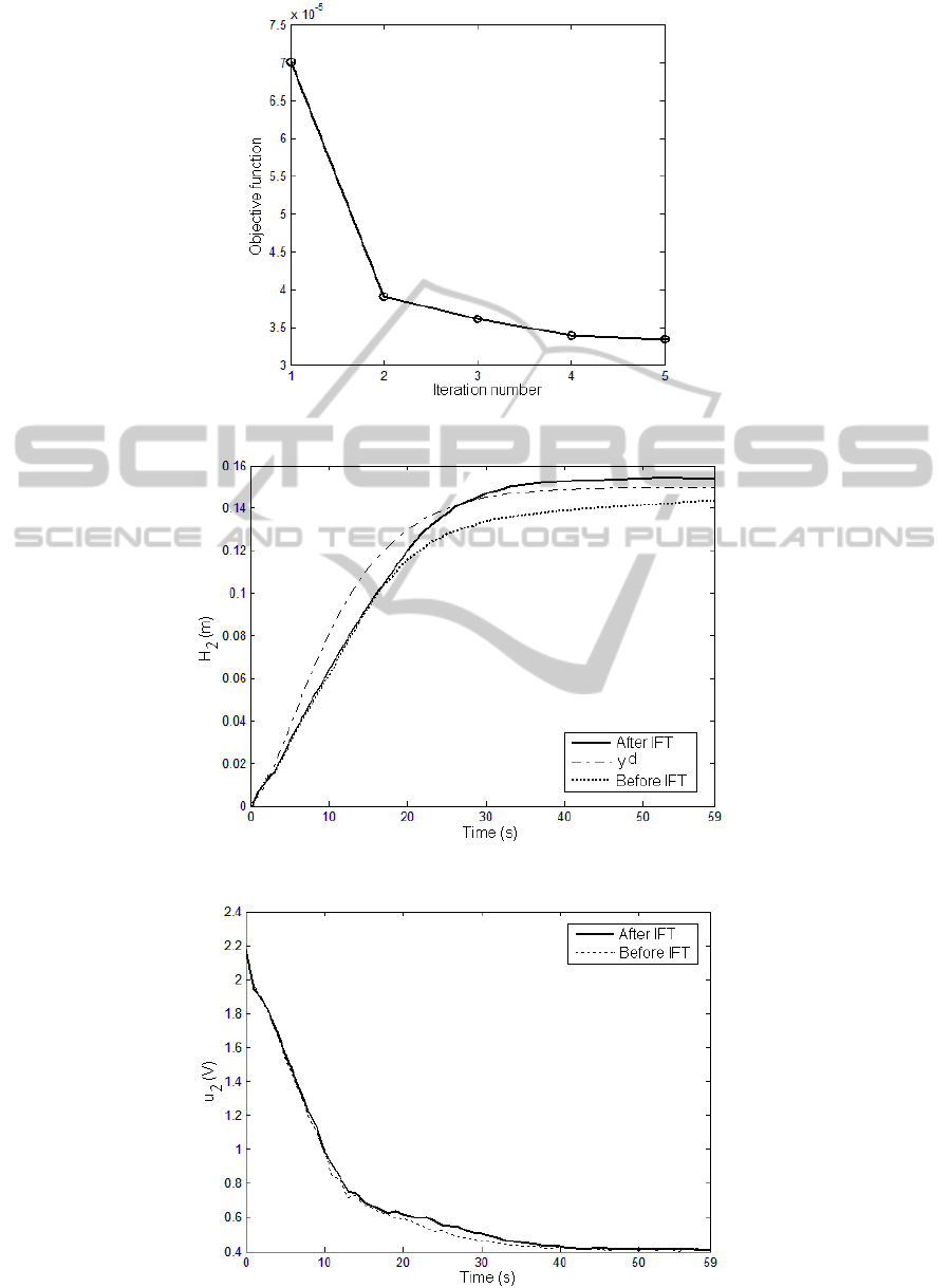
Figure 8: Objective function versus iteration number for control loop controlling H
2
.
Figure 9: Experimental results expressed as level H
2
versus time before and after IFT algorithm.
Figure 10: Experimental results expressed as control signal u
2
versus time before and after IFT algorithm.
Data-basedTuningofPIControllersforVerticalThree-TankSystems
37

6 CONCLUSIONS
This paper has suggested new IFT algorithms meant
for parameter tuning of PI controllers dedicated to
the level control of the first two tanks in vertical
three-tank systems. A complete data-based
experiment-based approach is proposed with this
regard.
The experimental results show that the six steps
of our IFT algorithms ensure the performance
improvement of a representative nonlinear MIMO
benchmark process. An improved model reference
tracking is observed after few iterations of IFT
algorithms. The control system structure presented
in this paper does not employ an adaptive model
reference approach.
The results concerning the control system
behaviour with respect to modifications of
disturbance inputs have not been presented. The
integral components of PI controllers ensure the
disturbance rejection.
One limitation of this data-based technique is the
need for initial PI stabilizing controllers tuned by a
model-based approach represented, for example, by
the MO method. The integral components of PI
controllers cope with the cross-couplings specific to
MIMO systems. However, different organizations of
the experiments specific to MIMO systems can be
applied in this context in order to ensure further
control system performance improvement (Sjöberg
et al., 2003; Huusom et al., 2009; Rădac et al., 2009;
McDaid et al., 2010; Precup et al., 2010).
Future research will be focused on other data-
based tuning techniques applied to nonlinear MIMO
systems and on comparison of the performance of
similar tuning techniques. Special gradient
experiments for MIMO systems should be
constructed with this regard in order to fit the normal
operating regimes of control systems.
ACKNOWLEDGEMENTS
This work was supported by a grant of the Romanian
National Authority for Scientific Research, CNCS –
UEFISCDI, project number PN-II-ID-PCE-2011-3-
0109, and by a grant of the NSERC of Canada.
REFERENCES
Ahmed, S., Petrov, M., Ichtev, A., 2010. Fuzzy model-
based predictive control applied to multivariable level
control of multi tank system. In Proceedings of 5
th
IEEE International Conference Intelligent Systems (IS
2010). London, UK, 456-461.
Antić, D., Nikolić, S., Milojković, M., Danković, N.,
Jovanović, Z., Perić, S., 2011. Sensitivity analysis of
imperfect systems using almost orthogonal filters.
Acta Polytechnica Hungarica. 8, 79-94.
Åström, K. J., Hägglund, T., 1995. PID Controllers
Theory: Design and Tuning. Research Triangle Park,
NC: Instrument Society of America.
Bazanella, A. S., Gevers, M., Miskovic, L., Anderson, B.
D. O., 2008. Iterative minimization of H
2
control
performance criteria. Automatica. 10, 2549-2559.
Bigher, B.-A., 2011. Iterative feedback tuning-based
control structures. Applications to a multi-tank system
laboratory equipment. B.Sc. thesis, Faculty of
Automation and Computers, “Politehnica” University
of Timisoara, Timisoara, Romania.
Blažič, S., Škrjanc, I., Gerkšič, S., Dolanc, G., Strmčnik,
S., Hadjiski, M. B., Stathaki, A., 2009. Online fuzzy
identification for an intelligent controller based on a
simple platform. Engineering Applications of Artificial
Intelligence. 22, 628-638.
Ferreira, P. M., Ruano, A. E., 2009. On-line sliding-
window methods for process model adaptation. IEEE
Transactions on Instrumentation and Measurement.
58, 3012-3020.
Giua, A., Seatzu, C., 2008. Modeling and supervisory
control of railway networks using Petri nets. IEEE
Transactions on Automation Science and Engineering.
6, 431-445.
Hjalmarsson, H., 1998. Control of nonlinear systems using
iterative feedback tuning. In Proceedings of 1998
American Control Conference (1998 ACC).
Philadelphia, PA, USA. 4, 2083-2087.
Hjalmarsson, H., 2002. Iterative feedback tuning - an
overview. International Journal of Adaptive Control
and Signal Processing. 16, 373-395.
Hjalmarsson, H., Gevers, M., Gunnarsson, S., Lequin, O.,
1998. Iterative feedback tuning: theory and Applica-
tions. IEEE Control Systems Magazine. 18, 26-41.
Hjalmarsson, H., Gunnarsson, S., Gevers, M., 1994. A
convergent iterative restricted complexity control
design scheme. In Proceedings of 33
rd
IEEE
Conference on Decision and Control. Lake Buena
Vista, FL, USA, 1735-1740.
Huusom, J. K., Poulsen, N. K., Jørgensen, S. B., 2009.
Improving convergence of iterative feedback tuning.
Journal of Process Control. 19, 570-578.
Iglesias, J. A., Angelov, P., Ledezma, A., Sanchis, A.,
2010. Evolving classification of agents’ behaviors: a
general approach. Evolving Systems. 1, 161-171.
Inteco, 2007. Multitank System, User’s Manual. Krakow,
Poland: Inteco Ltd.
Johanyák, Z. C., 2010. Student evaluation based on fuzzy
rule interpolation. International Journal of Artificial
Intelligence. 5, 37-55.
Kasabov, N., Hamed, H. N. A., 2011. Quantum-inspired
particle swarm optimisation for integrated feature and
parameter optimisation of evolving spiking neural
networks. International Journal of Artificial
ICINCO2012-9thInternationalConferenceonInformaticsinControl,AutomationandRobotics
38

Intelligence. 7, 114-124.
Kumar, N., Dhiman, R., 2011. Optimization of PID
controller for liquid level tank system using intelligent
techniques. Canadian Journal on Electrical and
Electronics Engineering. 2, 531-535.
Leva, A., Maggio, M., 2011. A systematic way to extend
ideal PID tuning rules to the real structure. Journal of
Process Control. 21, 130-136.
Linda, O., Manic, M., 2011. Uncertainty-robust design of
interval type-2 fuzzy logic controller for delta parallel
robot. IEEE Transactions on Industrial Informatics. 7,
661-670.
McDaid, A. J., Aw, K. C., Xie, S. Q., Haemmerle, E.,
2010. Gain scheduled control of IPMC actuators with
‘model-free’ iterative feedback tuning. Sensors and
Actuators A: Physical. 164, 137-147.
Nikolić, S., Danković, B., Antić, D., Jovanović, Z., 2010.
On identification of discrete systems. Facta
Universitatis, Series: Automatic Control and Robotics.
9, 59-67.
Orani, N., Pisano, A., Usai, E., 2010. Fault diagnosis for
the vertical three-tank system via high-order sliding-
mode observation. Journal of The Franklin Institute.
347, 923-939.
Petres, Z., Baranyi, P., Korondi, P., Hashimoto, H., 2007.
Trajectory tracking by TP model transformation: case
study of a benchmark problem. IEEE Transactions on
Industrial Electronics. 54, 1654-1663.
Precup, R.-E., Moşincat, I., Rădac, M.-B., Preitl, S.,
Kilyeni, S, Petriu, E. M., Dragoş, C.-A., 2010.
Experiments in iterative feedback tuning for level
control of three-tank system. In Proceedings of 15
th
IEEE Mediterranean Electromechanical Conference
(MELECON 2010). Valletta, Malta, 564-569.
Precup, R.-E., Tomescu, M. L., Rădac, M.-B., Petriu, E.
M., Preitl, S., Dragoş, C.-A., 2012. Iterative
performance improvement of fuzzy control systems
for three tank systems. Expert Systems with
Applications. DOI: 10.1016/j.eswa.2012.01.165.
Rădac, M.-B., Precup, R.-E., Petriu, E. M., Preitl, S.,
2011. Application of IFT and SPSA to servo system
control. IEEE Transactions on Neural Networks. 12,
2363-2375.
Rădac, M.-B., Precup, R.-E., Petriu, E. M., Preitl, S.,
Dragoş, C.-A., 2009. Iterative feedback tuning
approach to a class of state feedback-controlled servo
systems. In Proceedings of 6
th
International
Conference on Informatics in Control, Automation and
Robotics (ICINCO 2009). Milan, Italy, 1, 41-48.
Sjöberg, J., De Bruyne, F., Agarwal, M., Anderson, B. D.
O., Gevers, M., Kraus, F. J., Linard, N., 2003. Iterative
controller optimization for nonlinear systems, Control
Engineering Practice. 11, 1079-1086.
Tar, J. K., Rudas, I. J., Nagy, I., Kozlowski, K. R.,
Tenreiro Machado, J. A., 2009. Simple adaptive
dynamical control of vehicles driven by
omnidirectional wheels. In Proceedings of IEEE 7
th
International Conference on Computational
Cybernetics (ICCC 2009). Palma de Mallorca, Spain,
91-95.
Vaščák, J., Madarász, L., 2010. Adaptation of fuzzy
cognitive maps – a comparison study. Acta
Polytechnica Hungarica. 7, 109-122.
Data-basedTuningofPIControllersforVerticalThree-TankSystems
39
