Modeling and Active Vibration Control of a Smart Structure
Nader Ghareeb and R¨udiger Schmidt
Institute of General Mechanics, RWTH Aachen University of Technology, Templergraben 64, Aachen, Germany
Keywords:
Super Element Model, Lyapunov Function Controller, Strain Rate Feedback Controller.
Abstract:
Active vibration control of flexible structures has gained much attention in the last decades. The major com-
ponents of any active vibration control system are the mechanical structure suseptible to vibration, sensor(s) to
perceive it, actuator(s) to counteract the influence of disturbances causing vibration and finally, the controller
responsible for the generation of appropriate control signals. In this paper, a Lyapunov function controller and
a strain rate feedback controller (SRF) are used to attentuate the vibrations of a cantilivered smart beam excited
by its first eigenmode. A super element (SE) with a finite number of degrees of freedom (DOF) is derived from
the modified and damped finite element (FE) model. The state-space (SS) equations of the same model are
also extracted. Controllers are applied to the SE and SS models and results are presented and compared.
1 INTRODUCTION
In modern engineering, weight optimization has al-
ways the highest priority during the design of struc-
tures. Despite all its advantages, it results in lower
stiffness and less internal damping which cause the
structure to become more sensitive to vibrations
which could even lead to its failure (Ghareeb and
Radovcic, 2009). One way to overcome this prob-
lem is to implement active or smart materials that
can be controlled in accordance to the disturbances
or oscillations sensed by the structure itself. The cou-
pled electromechanical properties of smart materials,
which are used here in the form of piezoelectric ce-
ramics, make them well suited for the use as dis-
tributed sensors and actuators for controling structural
response. In the sensor application, mechanically in-
duced deformations can be determined from measure-
ment of the induced electrical potential, whereas in
actuator applications deformation or strains can be
controled through the introduction of an appropri-
ate electric potential (Narayanan and Balamurugan,
2003). Active vibration control has been applied at
the beginning on ships (Mallock, 1905), and later
on aircrafts (Hort, 1934). The rapid developments
in this field lead after that to the use of point actu-
ators and sensors to control flexible systems based
on the knowledge of elastic mode frequencies and
mode shapes at their location (Balas, 1978). The
use of piezoelectric materials as actuators and sen-
sors for noise and vibration control has been illus-
trated extensively over the past 30 years. An ac-
tive vibration damper for a cantilever beam using a
distributed parameter actuator was designed by (Bai-
ley, 1984). Three different control algorithms to con-
trol the cantilevered beam vibration with piezoactua-
tors were developed and implemented by (Bailey and
Hubbard, 1985). A rigorousstudy on the stress-strain-
voltage behavior of piezoelectric elements bonded to
beams was presented by (Crawley and de Luis, 1987)
and (Crawley and Anderson, 1990). Many other re-
searchers have also investigated the implementation
and use of piezoelectric actuators like (Fanson and
Chen, 1986), (Preumont, 2002), etc.
The present work comprises modeling of a smart
beam and the design of active linear controllers to
control its vibrations. The piezoactuator is initially
modeled and the relation between voltage and mo-
ments at its ends is examined. A modified FE model
of the smart beam is then created. The damping co-
efficients are calculated and added to it prior to the
reduction to a SE with a finite number of DOF. The
SS model is also extracted to check the controllers.
The FE- and SE models are validated by performing a
modal analysis and comparing the results to the exper-
imental ones. Finally, a Lyapunov function controller
and a SRF controller are introduced and implemented
on the SE and the SS models of the smart beam and
results are shown. The FE package SAMCEF is used
for the creation of the FE and the SE models, and
MATLAB-SIMULINK is used for the implementa-
tion of the controllers in the SS form.
142
Ghareeb N. and Schmidt R..
Modeling and Active Vibration Control of a Smart Structure.
DOI: 10.5220/0004004301420147
In Proceedings of the 9th International Conference on Informatics in Control, Automation and Robotics (ICINCO-2012), pages 142-147
ISBN: 978-989-8565-21-1
Copyright
c
 2012 SCITEPRESS (Science and Technology Publications, Lda.)

2 MODELING
The first step in designing a control system is to build
a mathematical model of the system and disturbances
causing the unwanted vibrations. The structural ana-
lytical model can be derived by using the FE method.
The smart structure used here consists of a steel beam,
a bonding layer and an actuator (Figure 1).
V
beam
actuator
bonding layer
Figure 1: The smart beam.
2.1 Actuator Modeling
The introduction of an actuator implies the imple-
mentation of an appropriate electric potential to
control the vibrations in the smart structure (converse
piezoelectric effect). The voltage applied can be
represented by two equal moments with opposite
directions concentrated at it’s ends (Fanson and Chen,
1986). The behavior of the piezoelectric material is
assumed to be linear thoughout this work. By consid-
ering the schematic layout of the middle portion of
the smart beam (Figure 2), if a voltage V is applied
across the piezoelectric actuator while assuming one
dimensional deformation, the piezo-electric strain ε
p
in the piezo is:
M
p
y
b
D
t
3
t
2
t
1
z
beam
actuator
bonding
x
z
M
p
Figure 2: A schematic layout of the composite beam.
ε
p
=
d
31
t
1
·V (1)
V is the voltage of the piezo-electric actuator, d
31
the
electric charge constant and t
1
it’s thickness.
The longitudinalstress can be expressed with Hooke’s
law as:
σ
p
= E
1
· ε
p
(2)
where E
1
is the Young’s modulus of the piezo
This stress generates a bending moment M
p
around
the neutral axis of the composite beam given by:
M
p
=
Z
(t
1
+t
2
+t
3
−D)
(t
2
+t
3
−D)
σ
p
· b· zdz (3)
By considering the equilibrium of moments about the
neutral axis:
Z
beam
σ
3
dA +
Z
adhesive
σ
2
dA +
Z
piezo
σ
1
dA = 0 (4)
the position of the neutral axis D is found.
Substituting D, (1) and (2) in (3) determines the bend-
ing moment generated by the piezo M
p
as a function
of the voltage V:
M
p
=
E
1
E
2
(t
1
t
2
+ t
2
2
) + E
1
E
3
(t
2
3
+ t
1
t
3
+ 2t
2
t
3
)
2(E
1
t
1
+ E
2
t
2
+ E
3
t
3
)
d
31
bV
Now, the actuator moment can be taken instead of
the voltage as input to the controllers that will be de-
signed and implemented.
2.2 FE Modeling of the Smart Beam
The resultant FE model of the smart beaam must be
faithfully representative so that it can be used for fur-
ther applications like control analaysis (He and Fu,
2001). In order to find the best FE model, the opti-
mal element type and size must be selected. Thus,
a modal analysis of the real beam is experimentally
performed and then the results are compared to those
from the FE with different element types used. A de-
tailed geometry of the smart beam is shown (Figure 3)
and the material properties and thickness of each part
are represented (Table 1).
layer
1307510
5
10
10
5
composite
Figure 3: A detailed geometry of the smart beam [dimen-
sions in mm].
Table 1: Parameters of the components of smart beam.
Beam Bonding Actuator
Material steel epoxy PIC 151
Thickness [mm] 0.5 0.036 0.25
Density [kg/m
3
] 7900 1180 7800
Young’s mod. [GPa] 210 3.546 66.667
ModelingandActiveVibrationControlofaSmartStructure
143

Table 2: Comparison between FE and SE models.
FE model Experiment
1
st
eigenfrequency [Hz] 13.81 13.26
2
nd
eigenfrequency [Hz] 42.67 41.14
2.2.1 FE - Type and Size
The smart beam is modeled as a composite shell with
three layers, but without any relative slip among the
contact surfaces. Hence, each layer has its own me-
chanical properties. To validate the element type
used, a modal analysis is done and the first two eigen-
frequencies are read and compared to those from the
experiment (Table 2).
Although reducing the element size can improve
the solution accuracy, but the use of excessively fine
elements may result in unmanageable computations
that exceed the memory capabilities of existing com-
puters (Ko and Olona, 1987). The analysis shows that
using an element size less than 1 mm doesn’t make
any significant change on the values of the 1
st
and 2
nd
eigenfrequencies of the smart beam.
2.2.2 Damping Characteristics
Damping parameters are of significant importance in
determining the dynmaic response of structures (Lee
and Davidson, 2004). In this work, the damping is as-
sumed to be viscous and frequency dependent for the
sake of convenience and simplicity. A special case
of viscous damping is known as the proportional or
Rayleigh damping. The damping matrix is thus ex-
pressed as a linear combination of mass and stiffness
matrices of the undamped model (Rayleigh, 1877):
C = αM + βK (5)
where α and β are real scalars that need to be de-
termined. To do that, many methods are available
(Spears and Jensen, 2009) and (Adhikari, 2000).
However, a method that was developed by (Chowd-
hury and Dasgupta, 2003) is used in this work.
3 THE SUPER ELEMENT
The main virtue of this technique is the ability to per-
form the analysis of a complete structure by using re-
sults of prior analysis of different regions comprising
the whole structure. Thus, all DOF considered useless
for the final solution will be condensed and the rest
will be retained. This means, the DOF of the whole
system will correspond to the retained nodes plus a
number of internal deformation modes. To construct
the SE, the component-mode method is used (Craig
and Bampton, 1968), (Rickelt-Rolf, 2009).
3.1 The Component-mode Method
also called method of Craig-Bampton, it implies that
the basic substructure is split into a certain number of
substructures. The DOF of each substructure are then
classified into boundary DOF and internal DOF. The
boundary DOF are shared by several substructures,
while the internal DOF belong only to the considered
substructure. The behavior of each substructure is de-
scribed by the combinationof two types of component
modes; the constrained modes and the normal vibra-
tion modes. The former are determined by assigning
a unit displacement to each boundary DOF while all
other boundaries DOF are being fixed. The latter cor-
respond to the vibration modes obtained by clamping
the structure at its boundary. It is thus assumed that
the behavior of the substructure in the global system
can be represented by superimposing the constrained
modes and a small number of normal modes. Hence,
by retaining only the low-frequency vibration modes,
the substructure’s dynamic deformed shape is repre-
sented with sufficient accuracy.
3.2 SE Modeling
In order to construct a SE, the retained nodes and the
condensed nodes must be designated and the num-
ber of internal modes to be used must be specified.
The retained nodes are usually those where boundary
conditions are applied, or where stresses, displace-
ments,...etc are applied or measured. Based on the
current work, 10 internal modes responding to about
95% participation of the mass are used and five re-
tained nodes are considered (Figure 4). Node 1 is
clamped, actuator moments are added on node 2 and
node 3. Node 4 is used as a secondary sensor (for fu-
ture works), and node 5 is used as a sensor to measure
the tip displacement. A comparison between the FE
and the SE models is shown in (Table 3) and (Table 4).
Results of modal analyses on both models don’t show
a big difference concerning the eigenfrequencies.
1 54
32
Figure 4: The retained nodes of the super element.
4 THE STATE SPACE MODEL
The fundamental equation describing the dynamic
ICINCO2012-9thInternationalConferenceonInformaticsinControl,AutomationandRobotics
144

Table 3: Characteristics of FE and SE models.
FE model SE model
Number of nodes 8206 5
Number of elements 2575 1
DOF 49236 34
Table 4: Comparison between the eigenfrequencies.
FE model SE model % Error
1
st
freq [Hz] 13.811 14.249 3.07
2
nd
freq [Hz] 42.673 43.414 1.71
behavior of a damped structure discretized by the FE
method is written in the form:
M ¨q(t) + C ˙q(t) + Kq(t) = f(t) (6)
where q(t) is the state vector which collects the dis-
palcements of the structure by DOF, and the f(t) vec-
tor expresses the applied loads. If the total number of
DOF of the FE model is n, then the dimension of the
state vector q(t) is also n, and that of the mass, stiff-
ness and damping matrices will be n ∗ n. However,
since a SE is constructed and the desired results only
concern specific locations of the structure, n will be
reduced to s. In this case:
s = r + m − 6 (7)
r and m are the number of retained nodes, and the
number of internal modes chosen.
The SS model is written according to (6) with dimen-
sions of the SE model. The general form is:
˙x = Ax + Bu, and y = Cx + Du (8)
x is the state vector, u and y are the input and output
vectors. By using a Fortran code, and upon specifying
the type and position of inputs and outputs, the SS
model of the SE model is created.
5 CONTROLLER DESIGN
The performance of smart structures for active vibra-
tion control depends strongly on the control algorithm
accompanied with it. The objective is to design con-
trollers capable of damping the vibrations due to the
first eigenmode of the smart beam. The beam is ini-
tially excited with its first eigenmode and then it is
left to vibrate freely. At this moment, the controllers
are activated. Two vibration suppression methods are
used; Lyapunov stability-based theorem control and
the SRF control.
5.1 Lyapunov Stability Theorem
Although there is no general procedure for construct-
ing a Lyapunov function, yet any function can be con-
sidered as a candidate if it meets some requirements,
i.e. positive definite, equal to zero at the equilib-
rium state and with its derivative less or equal to zero
(Khalil, 1996). Now, the energy equation of a thin
Bernoulli-Euler beam modeled as a single FE in a
one-dimensional system with length h and left point
coordinate x
i
, will be considered as a Lyapunov func-
tion candidate:
U =
1
2
Z
x
i+h
x
i

ρ

∂y
∂t

2
+ EI

∂
2
y
∂x
2

2

dx (9)
This function is locally positive definite, continuously
differentiable and equal to zero at the equilibrium
state. Yet, the derivative of this function must be
smaller or less than zero.
˙
U =
Z
x
i+h
x
i

ρ˙y¨y + EI
∂
2
y
∂x
2
∂
∂t

∂
2
y
∂x
2


dx (10)
Substituting the equations for the bending moment M
and shear forceV in a beam (Petyt, 2003) and assum-
ing there is no shear yields:
˙
U = M

˙
y′
x
i
+h
−
˙
y′
x
i

(11)
To ensure that (11) is always smaller or equal to zero,
the actuator moment M can have the value:
M = − k

˙
y′
x
i
+h
−
˙
y′
x
i

(12)
where k is a positive constant. Substituting (12) in
(11) yields:
˙
U = − k

˙
y′
x
i
+h
−
˙
y′
x
i

2
≤ 0 (13)
In this case, (12) can be used as the controller for the
smart beam.
5.1.1 SE Model with Controller
Based on the SE model created, two equal moments
at nodes 2 and 3 (but with opposite directions) are
added, where each one of them is a function of the
velocities at both nodes according to (12). The effec-
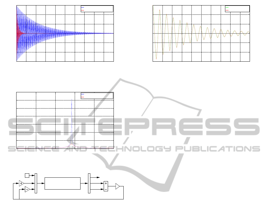
tiveness of this control strategy is shown in (Figure 5),
and its effect on the magnitude of the eigenmode on
the FFT spectrum diagram is illustrated in (Figure 6).
5.1.2 SS Model with Controller
In the SS, two steps are done. In step one, the only
input is the forced excitation with the first eigenmode
ModelingandActiveVibrationControlofaSmartStructure
145

20 22 24 26 28 30 32 34 36 38 40
−0.03
−0.02
−0.01
0
0.01
0.02
0.03
Time (s)
Tip displacement (m)
No control
Lyapunov stability theorem
Figure 5: Tip displacement vs. time with and without con-
troller during the free vibration (SE model is used).
0 5 10 15 20 25
0
0.01
0.02
0.03
0.04
0.05
0.06
0.07
Frequency (Hz)
Magnitude (mm)
No control
Lyapunov stability theorem
Figure 6: The FFT spectrum of the smart beam.
v
3
y = Cx + Du
x′ = Ax + Bu
Tip displacement
0
k
M
3
M
2
v
2
Figure 7: The SS model of the smart beam with controller.
and the output consists of the state vectors that are
fed as initial conditions for the second step. In step
two, (Figure 7), the input consists of both actuator
moments. The output comprises the tip displacement
at the 5
th
retained node, and the velocities at the 2
nd
node and 3
rd
node. Based on the Lyapunov stability
theorem, the output multiplied by a constant k is fed
back as actuator moments with different signs.
5.1.3 Comparison of Results from Both Models
The controller is implemented on both models and a
very slight difference is seen if the output curves are
zoomed (Figure 8). This is due to the fact that differ-
ent time steps are used in both models. Thus, using a
SE model decreases the simulation time and can show
more results (e.g. stresses, energy curves, etc).
5.2 Strain Rate Feedback Control
The SRF control can be used for active damping of
a flexible space structure (Fei and Fang, 2006). The
20 20.1 20.2 20.3 20.4 20.5 20.6 20.7 20.8 20.9 21
−0.03
−0.02
−0.01
0
0.01
0.02
0.03
Time (s)
Tip displacement (m)
SS control
SE control
Figure 8: Tip displacement vs. time with both models.
structural velocity coordinate is fed back to the com-
pensator, and the compensator position coordinate
multiplied by a negative gain is fed back to the struc-
ture. The SRF model can be presented with the fol-
lowing equations:
¨
ξ + 2ζ
˙
ξ + ω
2
ξ = − Gω
2
η (14)
¨
η + 2ζ
c
ω
c
˙
η + ω
c
η = ωc
2
˙
ξ (15)
ξ is the modal coordinate of structure displacement,
ζ is the damping ratio of the structure, ω is the
it’s natural frequency, G is the feedback gain, η
is the compensator coordinate, ζ
c
is the damping
ratio of the compensator and ω
c
it’s natural frequency.
Since all the parts of the smart beam are inter-
grated in a single SE, it is supposed that the smart
beam and the controller have the same damping
ratio and the same eigenfrequency. Applying this
assumption in the equation of the smart beam gives:
¨
ξ+ 2ζω
˙
ξ+ (ω
2
+ Gβω
2
)ξ = 0 (16)
In this case, there will be an increase in the stiffness
of the structure (active stiffness). However, the stabil-
ity condition is not clearly defined here due to the fact
that the closed-loop damping and stiffness matrices
of the whole system cannot be symmetrized (New-
man, 1992). The effectiveness of the SRF controller
is shown in (Figure 9). The magnitude of the eigen-
mode of the system decreases as well (Figure 10).
6 CONCLUSIONS AND FUTURE
WORK
In this work, the basic procedures for the modeling
and simulation of a smart beam were presented and
the SE and SS models were derived. A Lyapunov
function and a SRF controllers were designed and im-
plemented, and their effectiveness was checked.
In the future, an observer will be designed to count
for the geometrical nonlinearities which were not con-
sidered in this work. Nevertheless, more eigenmodes
ICINCO2012-9thInternationalConferenceonInformaticsinControl,AutomationandRobotics
146

20 22 24 26 28 30 32 34 36 38 40
−0.03
−0.02
−0.01
0
0.01
0.02
0.03
Time, (s)
Tip displacement, (m)
No control
SRF control
Figure 9: Tip displacement vs. time with the SRF controller.
0 5 10 15 20 25
0
0.01
0.02
0.03
0.04
0.05
0.06
0.07
Frequency (Hz)
Magnitude (mm)
No control
SRF control
Figure 10: The FFT spectrum of the smart beam.
will be controlled, and other control strategies (e.g.
positive position feedback, PID controllers...etc) will
be investigated and implemented.
REFERENCES
Adhikari, S. (2000). Damping Models for Structural Vibra-
tions. PhD thesis, Cambridge University.
Bailey, T. (1984). Distributed-parameter vibration con-
trol of a cantilever beam using a distributed-parameter
actuator. Master’s thesis, Massachusetts Institute of
Technology.
Bailey, T. and Hubbard, J. (1985). Distributed piezoelectric-
polymer active vibration control of a cantilever beam.
AIAA Journal of Guidance and Control, 6:605–611.
Balas, M. (1978). Active control of flexible systems. Jour-
nal of Optimization Theory and Applications, 25:415–
436.
Chowdhury, I. and Dasgupta, S. (2003). Computation of
rayleigh damping coefficients for large systems.
Craig, R. and Bampton, M. (1968). Coupling of substruc-
tures for dynamic analysis. AIAA Journal, 6:1313–
1319.
Crawley, E. and Anderson, E. (1990). Detailed models of
piezoceramic actuation of beams. Journal of Intelli-
gent Material Systems and Structures, 1:4–24.
Crawley, E. and de Luis, J. (1987). Use of piezoelectric
actuators as elements of intelligent structures. AIAA
Journal, 25:1373–1385.
Fanson, J. and Chen, J., editors (1986). Structural Control
by the use of Piezoelectric Active Members, volume 2
of Proceedings of NASA/DOD Control-Structures In-
teraction Conference. NASA. CP-2447.
Fei, J. and Fang, Y., editors (2006). Active Feedback Vibra-
tion Suppression of a Flexible Steel Cantilever Beam
Using Smart Materials. Proceedings of the First Inter-
national Conference on Innovative Computing, Infor-
mation and Control (ICICIC’06).
Ghareeb, N. and Radovcic, Y. (2009). Fatigue analysis of a
wind turbine power train. DEWI Magazin, 35:12–16.
He, J. and Fu, Z. (2001). Modal Analysis. Butterworth-
Heinemann.
Hort, H. (1934). Beschreibung und versuchsergebnisse aus-
gefhrter schiffsstabilisierungsanlagen. Jahrb. Schiff-
bautechnik Ges., 35:292–312.
Khalil, H. (1996). Nonlinear Systems. Prentice Hall, Madi-
son.
Ko, W. and Olona, T. (1987). Effect of element size on the
solution accuracies of finite-element heat transfer and
thermal stress analysis of space shuttle orbiter. Tech-
nical Memorandum 88292, NASA.
Lee, J. B. J. and Davidson, B. (2004). Experimental deter-
mination of modal damping from full scale testing. In
13th World Conference on Earthquake Engineering,
number 310, Vancouver, Canada.
Mallock, A. (1905). A method of preventing vibration in
certain classes of steamships. Teans. Inst. Naval Ar-
chitects, 47:227–230.
Narayanan, S. and Balamurugan, V. (2003). Finite element
modelling of piezolaminated smart structures for ac-
tive vibration control with distributed sensors and ac-
tuators. Journal of Sound and Vibration, 262:529–
562.
Newman, S. (1992). Active damping control of a flexible
space structure using piezoelectric sensors and actua-
tors. Master’s thesis, U.S. Naval Postgraduate School,
California.
Petyt, M. (2003). Introduction to Finite Element Vibration
Analysis. Cambridge University Press.
Preumont, A. (2002). Vibration Control of Active Struc-
tures, An Introduction. Kluwer Academic Publishers.
Rayleigh, L. (1877). Theory of Sound, volume 1, 2. Dover
Publications, New York.
Rickelt-Rolf, C. (2009). Modellreduktion und Substruk-
turtechnik zur effizienten Simulation dynamischer
teilgesch¨adigter Systeme. PhD thesis, TU Carolo-
Wilhelmina zu Braunschweig, Germany.
Spears, R. and Jensen, S., editors (2009). Approach
for Selection of Rayleigh Damping Parameters Used
for Time History Analysis, Proceedings of PVP2009,
ASME Vessels and Piping Division Conference,
Prague, Czech Republic.
ModelingandActiveVibrationControlofaSmartStructure
147