
Load-following Control of APR+ Nuclear Reactors
Jae Hwan Kim
1
, Man Gyun Na
1
, Keuk Jong Yu
2
and Han Gon Kim
2
1
Department of Nuclear Engineering, Chosun University, 309 Pilmun-daero, Dong-gu, Gwangju, Korea
2
KHNP-Central Research Institute, 1312 Gil, 70. Yuseong-daero, Yuseong-gu, Daejeon, Korea
Keywords: Load-following Operation, Model Predictive Control, APR+ Reactor, Thermal Power Level, Axial Shape
Index (ASI), KISPAC-1D Code.
Abstract: The load-following operation of APR+ reactor is needed to control the power effectively using the control
rods and to restrain the reactivity control from using the boric acid for flexibility of plant operation. The
xenon has a very high absorption cross-section and makes the impact on the reactor delayed by the iodine
precursor. The power maneuvering using automatically load-following operation has advantage in terms of
safety and economic operation of the reactor. Therefore, an advanced control method that meets the
conditions such as automatic control, flexibility, safety, and convenience is necessary to load-following
operation of APR+ reactor. In this paper, the MPC method is applied to design APR+ reactor’s automatic
load-following controller for the integrated average coolant temperature and ASI control. The KISPAC-1D
code, which models the APR+ nuclear power plants, is interfaced to the proposed controller to verify the
tracking performance of the average coolant temperature and ASI. It is known that the proposed controller
exhibits very fast tracking responses.
1 INTRODUCTION
The performance of load following operation on a
nuclear power plant has been assessed differently
depending on the need for age and regional energy
environment. Now that nuclear power has emerged
as the most realistic alternative when fossil-fuel
prices increasing and global warming problem has
become a serious globally, nuclear power plant
construction plans have been announced in many
countries, and in case of Korea, also plan to increase
the share of nuclear power. So, it is difficult to
maintain the electric power demand by controlling
the power of only hydro and fossil power plants that
have the relatively low impact on an overall power
system. APR+ is a nuclear reactor which has the
power more than 1500MWe under development in
Korea. Dynamics of a nuclear power plant depends
on the reactivity changes according to the operating
conditions and fuel combustion. Thus, the reactor
power must be controlled well to maintain the
integrity of the nuclear power plant and to maximize
the thermal efficiency. Most of the existing nuclear
power plants change operating power by controlling
boron concentration in the coolant. However, the use
of boric acid is difficult to respond quickly to
demand for power changes, and it is limited for
usage at the end of a nuclear fuel cycle due to the
concern of a positive temperature coefficient. In case
of using the control rods, reactivity control can be
easier through the feedback of coolant for automatic
control, but power distribution control is very
complex due to nonlinear dynamic characteristics.
In this study, model predictive control (MPC)
technique is applied to design the automatic load
following controller for controlling the average
coolant temperature and axial shape index (ASI) of
APR+ reactors. The model predictive controller can
accomplish better tracking performance because it
considers not only the trace command of current
time but also future time. MPC technique has been
applied to many industrial process systems, and its
performance was also proven. The objectives of the
proposed MPC are to minimize the difference
between the estimated output (average coolant
temperature and ASI) and the desired output and the
frequent variation of the control rod position. And
KISPAC-1D code is interfaced to the proposed
controller to verify its performance for controlling
average coolant temperature and ASI.
446
Kim J., Na M., Yu K. and Kim H..
Load-following Control of APR+ Nuclear Reactors.
DOI: 10.5220/0004006604460451
In Proceedings of the 9th International Conference on Informatics in Control, Automation and Robotics (ICINCO-2012), pages 446-451
ISBN: 978-989-8565-21-1
Copyright
c
2012 SCITEPRESS (Science and Technology Publications, Lda.)
2 LOAD-FOLLOWING
OPERATION
Load following operation of a nuclear power plant
means the operation mode that reactor power
follows the load variation of the turbine. Daily load
following operation, frequency control operation,
and contingency power change operation belong to
the category of the load following operations. Daily
load following operation means that reactor power is
retained for a period of time as a constant rate of
change by up to 50%, and then return to 100%
power as a constant speed. However, the frequency
control operation of nuclear power plants causes the
frequent movement of control rods because of the
volatility of an ever-changing power system.
Therefore, the purpose of controller development
was set up to design the controller capable of daily
load following operation. Reactor power fluctuation
can be achieved by regulating the parameters that
cause the change of core reactivity. Core reactivity is
affected by changes of the boron concentration, fuel
and coolant temperature, xenon and samarium
concentration in the core.
Xenon and samarium concentrations are
excluded from the direct target which can be
controlled because it cannot be measured directly
during reactor operation, and fuel consumption rate
and fuel temperature are already determined in the
time of fuel loading. Control rod movement can be
used as a control factor for immediate reactor power
changes because it impacts on the reactor within a
few seconds, and the change of boron concentration
in the coolant should be used essentially to control
the surplus reactivity since it is affected to the
reactor within few minutes. Coolant temperature can
be used as a control factor which reduces the use of
control rods and boron.
3 DESIGN OF MODEL
PREDICTIVE CONTROLLER
The average coolant temperature and reactor power
distribution should be controlled at the same time for
load following operation. The MPC controller is
introduced for the automatically load following
operation of an APR+ reactor. It uses a control
method that can perform optimal control with the
predictive calculations. Through this study, an MPC
controller will be designed so that it can control the
average coolant temperature and power distribution
at the same time.
3.1 Basic Principle of MPC
MPC method can calculate control input of the
constant horizon by solving the optimization
problems about finite future time steps in the current
time, and actually implement solely the first optimal
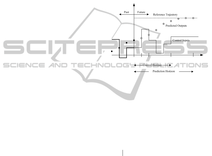
input as a control input. As shown in the Figure 1,
new output is measured at the next time step, and
control horizon moves one step forward, and these
calculations are repeated.
t
1t
+
tM+
tP+
LL
ˆ
(|)
y
tkt+
()ut k
+
w
Figure 1: Concept of the Model Predictive Control.
The purpose of using a new measured value at
each time step is to compensate the model
inaccuracy or unmeasured disturbance. The basic
elements of MPC contain a specific model
(prediction model) for predicting the process output
of a point in the future, an objective functions and its
optimization.
Using this prediction model, outputs for the
prediction horizon
P ,
ˆ
[( |), 1,2, , ]tktk P+=y
L
are predicted, and these outputs depend on the past
input, output and future input (control signal),
[( ), 1,2, , ]tktk M+=u L
.
A series of optimal control signal is calculated by
optimizing a given objective function to let the
output follow the target output as fast as possible. In
case the objective function is quadratic form, and the
model is linear, and constraint does not exist, the
control input can be derived analytically. However
the actual control input in most of the processor
is obtained numerically. At this time, the optimal
control input is obtained in a range which satisfies
the constraints by including the constraint which will
be applied to the system to the
algorithm. Among the optimized control signals, the
first input
(/)ttu is sent only to the process input.
And the remaining control input signals are
meaningless because
(1)t
+
y
was already known in
Load-followingControlofAPR+NuclearReactors
447

the next sampling period. So, control input is
calculated newly by repeating the previous
procedure for every sampling period. Performance
indicator can be written to obtain a fast response and
to prevent excessive control effort as follows:
1
1
1
ˆ
ˆ
(( |) ( ))Q(( |)
2
1
( )) ( 1) R ( 1)
2
P
T
k
M
T
k
Jtkttktkt
tk tk tk
=
=
=+−+ +
−++ Δ+− Δ+−
∑
∑
ywy
wuu
(1)
the constraints are:
ˆ
()(),1,,
(1)0, ()
tPi tPi i L
t k k M M P
++= ++ =
⎧
⎨
Δ+−= > <
⎩
yw
u
L
(2)
where
ˆ
()tkt+y
is k-step-ahead optimal prediction
of the system based on data until the current time
t
. And
w
indicates a series of output set point vector,
and
Δu
is the control input change between two
neighboring time steps. Positive definite matrices
Q
and
R are symmetric matrices that it gives each
weight to the particular component of
ˆ
()
−
y
w
and
Δu
in some future time horizon.
The number of output has two, and they consist
of average coolant temperature and ASI. And the
number of input has also two. These indicate the
axial position of two types of control banks
(regulating control bank, part-strength control bank).
Usually,
P is called a prediction horizon, and
M
is called a control horizon. Prediction horizon
means limited time intervals to follow the output on
the demand output. It has two constraints. The
constraint,
ˆ
()(), 1,,tPi tPii L++= ++ =yw
L ,
which makes the output follow the reference input
over some range and guarantees the stability of the
controller.
(1)0,
tk k MΔ+−= >u
means that
there is no variation in the control signals after a
certain interval
()
M
P<
, which is the control
horizon concept.
3.2 Future Output Prediction
In the case of dynamic systems, future output
behavior can vary depending on the input of past,
present and future. Thus, past inputs should be
remembered in some forms for the prediction.
Dynamic states can be defined as a memory about
the past inputs that is necessary to predict the future
output behavior. States can be defined in many other
ways in the same system.
In case of a finite impulse response (FIR)
system, it is sufficient to keep
P
past inputs alone:
() [( 1),( 2), ( )]
T
x
kk k kP
υυ υ
=− − −L
(3)
The future output behavior can be definitely
predicted by selecting
()
x
k
. The ultimate goal of the
memory is to predict the future output, so the past
can be tracked more easily in terms of its effect on
the future than the past itself. In linear systems, the
effect on the past and (hypothesized) future inputs
can be calculated separately and added through the
principle of separation.
0
()Yk
is defined as future
output deviation due to past input deviation:
00 0 0
()[(/),( 1/),,(/)]
T
Yk ykkyk k y k=+∞L
(4)
where
0
(/ ) ()yik yi
assuming
()0
kj
υ
+=
for
0j ≥
Even if
0
()Yk
is infinite dimensional, for an FIR
system, it needs to keep only
P terms:
00 0 0
()[(/),( 1/),,(/)]
T
Yk ykkyk k yPk=+L
(5)
This vector can be chosen as the states because it
describes the effects of the past input deviation on
the future output deviation. Future output can be
written as:
0
0
0
0
Effect of Past Inputs From ( )
1
21
11
(1)
(1/)
(2)
(2/)
()
(/)
00
0
() ( 1)
Yk
PP
yk
yk k
yk
yk k
yk P
yk Pk
H
HH
kk
HH H
υυ
−
+
⎡⎤
+
⎡⎤
⎢⎥
⎢⎥
+
+
⎢⎥
⎢⎥
⎢⎥
⎢⎥
=
⎢⎥
⎢⎥
⎢⎥
⎢⎥
⎢⎥
⎢⎥
+
+
⎣⎦
⎣⎦
⎡⎤ ⎡ ⎤ ⎡⎤
⎢⎥ ⎢ ⎥ ⎢
⎢⎥ ⎢ ⎥ ⎢
⎢⎥ ⎢ ⎥ ⎢
++ +++
⎢⎥ ⎢ ⎥ ⎢
⎢⎥ ⎢ ⎥ ⎢
⎢⎥ ⎢ ⎥ ⎢
⎣⎦ ⎣ ⎦ ⎣
M
M
M
M
1442443
LMM M
MM M
Effect of Hypothesized Future Inputs
(1)kP
υ
⎥
⎥
⎥
+−
⎥
⎥
⎥
⎦
1
4444444444244444444443
(6)
This equation shows that the definition of the states
can be very convenient for the predictive control.
For computer implementation, the memory should
be updated in a recursive manner from one time step
to next.
0
()Yk
can be updated recursively as
follows:
ICINCO2012-9thInternationalConferenceonInformaticsinControl,AutomationandRobotics
448

000 0
00
00
00
00
( ) ( ) + ( ) = ( 1)
(/) ( 1/)
( 1/) ( 2/)
( 2/) ( 1/)
(1/) (/)
Yk Yk Hvk Yk
ykk yk k
yk k yk k
yk P k yk P k
yk P k yk Pk
→Ω +
⎡⎤⎡⎤
+
⎢⎥⎢⎥
++
⎢⎥⎢⎥
⎢⎥⎢⎥
→
⎢⎥⎢⎥
⎢⎥⎢⎥
⎢⎥⎢⎥
+− +−
⎢⎥⎢⎥
+− +
⎢⎥⎢⎥
⎣⎦⎣⎦
MM
MM
0
1
0
2
0
1
0
(1/ 1)
(2/1)
()
(1/1)
(/1)
P
P
H
yk k
H
yk k
k
H
yk P k
H
yk Pk
υ
−
⎡⎤
++
⎡⎤
⎢⎥
⎢⎥
++
⎢⎥
⎢⎥
⎢⎥
⎢⎥
+=
⎢⎥
⎢⎥
⎢⎥
⎢⎥
⎢⎥
⎢⎥
+− +
⎢⎥
⎢⎥
++
⎢⎥
⎢⎥
⎣⎦
⎣⎦
M
M
M
M
(7)
The above equation can be expressed as follows:
0
1
2
00
1
010 0
001 0
(1) () ()
000 1
000 0
P
P
H
H
Yk Yk k
H
H
υ
−
Ω
⎡⎤
⎡⎤
⎢⎥
⎢⎥
⎢⎥
⎢⎥
⎢⎥
⎢⎥
+= +
⎢⎥
⎢⎥
⎢⎥
⎢⎥
⎢⎥
⎢⎥
⎣⎦
⎣⎦
L
L
M
MMMOM
L
L
14442 4 4 43
(8)
The multiplication by
0
Ω in Eq. (8) represents the
shift operation which can be implemented efficiently
on the computer.
3.3 Added Constraint Conditions
In this paper, some constraints have been added, so
the control algorithm of MPC methodology has been
modified. The control system outputs are a coolant
average temperature (average coolant temperature)
and ASI. The control inputs are the two types of
control rod positions (considering long-term, short-
term steady-state insertion limits).
max
min
max
min
max max
() ,
() ,
() .
t
t
dtd
⎧
⎪
⎪
⎨
⎪
⎪
⎩
≤≤
≤≤
−≤Δ≤
yyy
uuu
uuu
(9)
The limited range of average coolant temperature is
1
290 315
oo
Cy C≤≤
, and the limited range of ASI
is
2
0.27 0.27y−≤≤
. Control inputs are control rods
position and speed (R5 position, P1&P2 positions).
Considering the short-term and long-term steady-
state insertion limits, the R5 control rod position is
limited within
1
152.4 381cm u cm≤≤ . The P1&P2
control rod position limit is
2
190.5 381cm u cm≤≤
.
Five types of a signal (high-speed insertion, low-
speed insertion, stop, low-speed withdrawal, high-
speed withdrawal) are used as the control rod speed
that is adjusted by the rod speed program. The
control rod speed of R5 and P1&P2 is 1.27 cm/sec
for high-speed insertion or withdrawal and 0.127
cm/sec for low-speed insertion or withdrawal, and 0
for stop. In this study, P1&P2 is moving together.
4 APPLICATION TO NUCLEAR
REACTOR POWER CONTROL
Load following operation control is considered an
MIMO (Multiple Input and Multiple Output) control
problem because the average coolant temperature
and ASI (Axial Shape Index) should be controlled
simultaneously. Load following operation is a two-
input and two-output system using the regulating
control bank and part-strength control bank as input
and the average coolant temperature and power
distribution as output.
This system can be expressed as follows:
111121
221222
() () () ()
() () () ()
y
kGqGquk
y
kGqGquk
⎡
⎤⎡ ⎤⎡ ⎤
=
⎢
⎥⎢ ⎥⎢ ⎥
⎣
⎦⎣ ⎦⎣ ⎦
(10)
From the above matrix,
11
()Gq
can be represented
by a discrete-time transfer function as follows:
1
01
1
01
()
n
d
n
n
n
bbq bq
Gq q
aaq aq
−−
−
−−
+++
=
+++
L
L
(11)
where
d is an integer (
0≥
) and represents the
sampling periods of pure delay.
Eq. (10) can be represented by a discrete
function as follows:
11112
22122
111 2
2212
() () () () () () ()
() () () () () () ()
dn n
dnn
yk qyk quk quk
yk qyk quk quk
θθθ
θθθ
=++
=++
(12)
1
()yk means the average coolant temperature and
2
()yk
means the power distribution (ASI). Adjusted
parameters in the numerical simulation are the
prediction horizon
P
, the control horizon
M
, and
the input weighting factors
1
μ
and
2
μ
of regulating
control bank R5 and part-strength control bank P,
respectively. To consider the constraints of MPC
controller systematically, a new MPC algorithm is
needed, and the control algorithm is required to be
interfaced with KISPAC-1D code that models the
reactor core dynamics and thermo-hydraulic parts.
Load-followingControlofAPR+NuclearReactors
449
The control algorithm was coded using MATLAB.
KISPAC-1D coded with the FORTRAN language is
needed to be interfaced with the MPC controller
programmed with MATLAB. Therefore, KISPAC-
1D code was converted into a library file using the
latest FORTRAN compiler to be integrated with the
control algorithm. To evaluate the load following
operation capability of the APR+ reactor using the
MPC method, we performed various simulations
using the KISPAC-1D code. The purpose of
simulation is to evaluate how well the average
coolant temperature and power distribution of the
reactor are controlled for a daily-load following
operation.
Daily-load following operation has a load cycle
of typical 100-50-100%, and power increasing
/decreasing speed is 25%/hr. We performed
simulations such as the following load change: 100-
50-100% power operation during a period of 24
hours. And the following initial conditions were
used in the numerical simulation. The initial reactor
power is 100%, regulating control bank (R5)
position is 370cm, other regulating control bank
position is 381cm, part-strength control bank (P)
position is 370cm, sampling period (T) is 4sec, bank
maximum speed is 1.27T cm/time step, prediction
horizon (
P ) is 5, control horizon (
M
) is 2, first
input weighting factor (
1
μ
) is 10, and second input
weighting factor (
2
μ
) is 30.
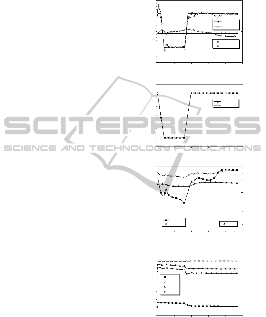
Figure 2 shows the results of numerical
simulation for daily-load following operation at the
beginning of a reactor fuel cycle. As shown in this
Figure 2(a), average coolant temperature are
different slightly from the desired temperature in the
power changed interval, but it follows desired
average coolant temperature in other sectors
according to target power level, and the tracking
performance of ASI shows that calculated ASI
doesn’t follows desired ASI perfectly. As shown in
the Figure 2(b), the calculated power level follows
the desired power level well. Figure 2(c) shows the
position of the regulating control bank and the part-
strength control bank and also shows the
concentration of boric acid. The rate of change of
the concentration of boric acid does not exceed the
boric acid capacity of the CVCS. Figures 2(d) and
(e) show that the parameters of
1
()q
θ
and
2
()q
θ
is
predicted repeatedly every time step, and show that
dynamic characteristic of the reactor changes
depending on the power level and the positions of
the control rod banks.
(
a) average coolant temperature and ASI
(b) reactor power level
(c) control rod bank position and boron concentration
(d)
1
()q
θ
polynomial
Figure 2: Simulation Results for Daily-Load Following
Operation.
0 5 10 15 20 25
301
302
303
304
305
306
307
308
309
310
311
0 5 10 15 20 25
-0.3
-0.2
-0.1
0.0
0.1
0.2
0.3
0.4
0.5
T
avg
(
o
C)
time (hr)
desired T
avg
T
avg
ASI
time (hr)
desired ASI
ASI
0 5 10 15 20 25
0.4
0.5
0.6
0.7
0.8
0.9
1.0
1.1
relative power
time
(
hr
)
demand load
core power
0 5 10 15 20 25
0
100
200
300
400
control rod position (cm)
time
(
hr
)
R5 position
P position
0
200
400
600
800
1000
boron
boron concentration (ppm)
0 5 10 15 20 25
-1.5
-1.0
-0.5
0.0
0.5
θ
1
(q) polynomial
time
(
hr
)
θ
1
(1,1)
θ
1
(1,2)
θ
1
(1,14)
θ
1
(1,15)
ICINCO2012-9thInternationalConferenceonInformaticsinControl,AutomationandRobotics
450

(e)
2
()q
θ
polynomial
Figure 2: Simulation Results for Daily-Load Following
Operation (Cont.).
5 CONCLUSIONS
In this study, we developed a new MPC algorithm
that can control the average coolant temperature and
axial power distribution systematically for load
following operation. The proposed controller was
applied to ensure the possibility of the load
following operation of APR+ reactor simulated
numerically by KISPAC-1D code. And a controller
design model used for designing the model
predictive controller is estimated every time step by
applying a parameter estimation algorithm to reflect
the time-varying condition. We examined the
performance of the controller by performing
numerical simulation at the beginning of the fuel
cycle. Through this study, we could see that the
average coolant temperature follows the desired
average coolant temperature well, but ASI tracking
performance is not good. It was hard to control the
average coolant temperature and ASI precisely at the
same time using two similar types of the control rods
because the dynamic characteristics of a regulating
control rod bank R5 is not much different from that
of the PSCEA. Through further study, we will
improve the performance of a model predictive
controller.
REFERENCES
Na, M. G., Jung, D. W., Shin, S. H., Jang, J. W., Lee, K.
B. and Lee, Y.J., Aug. 2005, A Model Predictive
Controller for Load-Following Operation of PWR
Reactors, IEEE Trans. Nucl. Sci., No. 52, pp. 1009-
1020.
Na, M. G., Feb. 2001, A Model Predictive Controller for
the Water Level of Nuclear Steam Generators, Nucl.
Eng. Tech., Vol. 33, No. 1, pp. 102-110.
Camacho, E. F., Bordons, C., 1999. Model Predictive
Control, Springer-Verlag, London.
MathWorks, MATLAB 5.3 (Release 11), 1999, The
MathWorks, Natick, Massachusetts.
Lee, J. W., Kwon, W. H., Choi, J., 1998, On Stability of
Constrained Receding Horizon Control with Finite
Terminal Weighting Matrix, Automatica, Vol. 34, No.
12, pp. 1607-1612.
Lee, J. W., Kwon, W. H. and Lee, J. H., 1997, Receding
Horizon
H
∞
Tracking Control for Time-Varying
Descrete Linear Systems, Intel. J. Control, Vol. 68,
No. 2, pp. 385-399.
Lee, Y. J., Choi, J. I., 1997, Robust Controller Design for
the Nuclear Reactor Power Control System, Nucl. Eng.
Tech., Aug. Vol. 29, pp. 280-290.
Kothare, M. V., Balakrishnan, V. and Morari, M., 1996,
Robust Constrained Model Predictive Control using
Linear Matrix Inequality, Automatica, Vol. 32, No. 10,
pp. 1361-1379.
Morari, M., Lee, J. H., 1999, Model Predictive control:
Past, present and future, Comp. and Chem., Eng., Vol.
23(4/5), pp. 667-682.
0 5 10 15 20 25
-1.5
-1.0
-0.5
0.0
0.5
θ
2
(q) polynomial
time
(
hr
)
θ
2
(1,1)
θ
2
(1,2)
θ
2
(1,14)
θ
2
(1,15)
Load-followingControlofAPR+NuclearReactors
451
