
Modeling and Simulation of a Wastewater Pumping Plant
Mohamed Abdelati
Electrical Engineering Department, IUG, Gaza, Palestine
Felix Felgner, Georg Frey
Chair of Automation, Saarland University, Saarbrücken, Germany
Keywords: Wastewater System Modeling, Simulation, Automation, Modelica.
Abstract: Modeling wastewater pumping plants is rarely addressed in the literature. Standard component models as
found in fluid simulation tool libraries are too complex, due to their projected generality, to be used for
these applications. Lack of models results in a burden on engineers who have to test their control scenarios
on real implemented systems. This may lead to unexpected delays and painful costs. In this work, easily
manageable component-oriented models are derived and applied to the modeling and simulation of a real
wastewater pumping system. The model derived in this paper is implemented in Modelica, and it helps
better understanding the system dynamics. Thereby, a tool is provided for evaluating the performance of
possible control schemes.
1 INTRODUCTION
Daily amounts of about 15000 m
3
of partially treated
wastewater are pumped through the new terminal
pumping station (NTPS) located at northern Gaza to
the new wastewater treatment plant (WWTP). Once
the construction of a new treatment plant is
completed, the pumping rate will reach an average of
35000 m
3
per day. The transmission pipe has 7.6 km
length, 80 cm diameter and 26 m static head. At the
present phase a group of ponds near the pumping
station are used to buffer and partially treat the
wastewater collected from northern Gaza (Werner et
al., 2006). Operators of the pumping station manually
control the intake amount of these ponds and allow it
to be pumped to the wastewater treatment plant. The
manual operation should be replaced by an
automation system. To this end, models for
evaluating different control schemes are necessary.
These models should allow efficient simulation of the
overall system over long time horizons, to validate
the system behavior especially under abnormal
conditions like e.g. power outages which are quite
common in Gaza.
The pumping station is equipped with 5 booster
pumps from ABS. Each pump has a power rating of
315 kW and an expected head of 38 m. It has a
pumping capacity of 360 kg/s while running safely at
a maximum speed of 1300 rpm. The suction chamber
of the booster pumps has a capacity of 500 m³ and
equipped with a level transmitter which is used to
control the operation of the booster pumps (Abdelati
and Rabah, 2007).
In (Abdelati et al., 2011) a model of the
wastewater recovery system was developed. The
work presented here, continues the project by
presenting a component-oriented model of the
wastewater pumping plant. The control scheme of the
pumping process will be detailed in Section 2 and
modeled in Section 3. The simulation results will be
presented in Section 4 and finally in Section 5,
concluding remarks will be given.
2 FUNCTIONAL DESCRIPTION
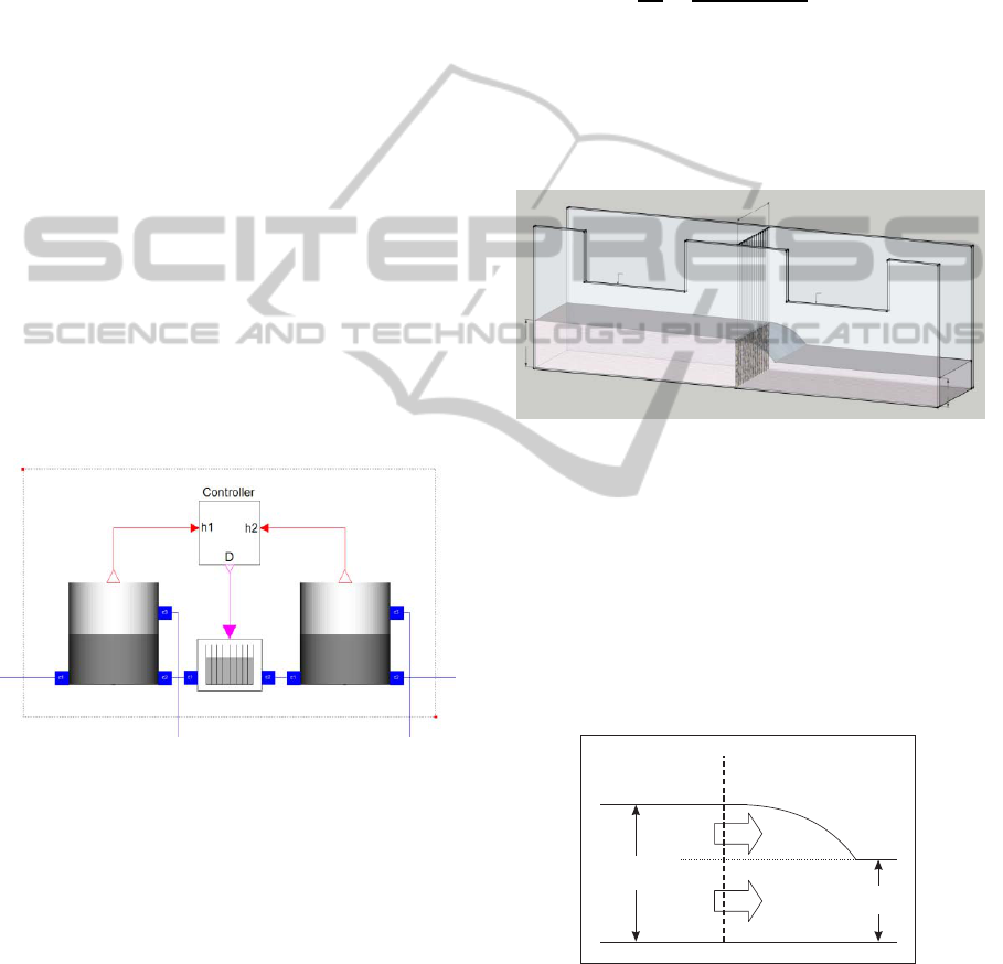
The new terminal pumping station (cf. process flow
diagram in Figure 1) transports wastewater from the
northern part of Gaza city to the new wastewater
treatment plant for Northern Gaza. It basically
consists of a screen station and a pump station
(Palestinian Water Authority, 2004).
377
Abdelati M., Felgner F. and Frey G..
Modeling and Simulation of a Wastewater Pumping Plant.
DOI: 10.5220/0004009803770384
In Proceedings of the 9th International Conference on Informatics in Control, Automation and Robotics (ICINCO-2012), pages 377-384
ISBN: 978-989-8565-21-1
Copyright
c
2012 SCITEPRESS (Science and Technology Publications, Lda.)

Figure 1: New terminal pumping station (NTPS).
2.1 Screen Station
The screen chamber receives the wastewater from
the pond by gravity force. The manual valve (V1)
allows setting the intake flow rate. The screen
separates coarse material out of wastewater. The
coarse material is loaded into a conveyor system.
The rack screen and the conveyor starts at a signal
due to difference in levels of level transmitters
(LT1) and (LT2) located in front of and behind the
screen respectively. They run during a preset time to
leave at pause position.
If the outtake of the screen fails to compensate
the intake, wastewater starts to accumulate in the
screen chamber. Overflow occurs if accumulation
reaches a specific level (1.6 m). The overflow is
collected in a dedicated pond where it is recharged
to the main pond by a minor process that is not
addressed in this paper.
2.2 Pump Station
This station pumps the wastewater from the suction
chamber to the new wastewater treatment plant. The
bottom of the suction chamber is placed 2.3 m below
the bottom of the screen chamber. The booster
pumps are controlled and operated by a signal from
level transmitter (LT3). Due to efficiency concerns,
pumps are not allowed to run at speeds below one
third their nominal speeds. The first pump in
operation starts at level L6. When one pump is in
operation, a flow of about 120-360 kg/sec
(corresponding to 33-100% rotational speed) will be
pumped using the frequency converter to keep a
preset value of the level (L5) in the suction chamber.
The first pump stops at level L1.
If the first pump operates at 100% capacity and
the level increases, the second pump starts at level
L7. When two pumps are in operation, a flow of
about 360-720 kg/s (corresponding to 50-100%
rotational speed) will be pumped using the
frequency converters to keep a preset value of the
level (L5) in the suction chamber. Each pump in
operation will pump 180-360 kg/s equal. The second
pump stops at level L3.
If two pumps operate at 100% and the level
increases up to level L8, the third pump starts. When
three pumps are in operation, a flow of about 720-
1000 kg/s (corresponding to 66-100% rotational
speeds) will be pumped using the frequency
converters to keep a preset value of the level (L5) in
the suction chamber. Each pump in operation will
pump 240-333 kg/s. The third pump stops at level
L3.
If three pumps operate at 100% and the level
increases up to level L9 the forth pump starts. When
four pumps are in operation, a flow of about 1000-
1200 kg/s (corresponding to 75-100% rotational
speeds) will be pumped using the frequency
converters to keep a preset value of the level (L5) in
the suction chamber. Each pump in operation will
pump 250-300 kg/s. The forth pump stops at level
L4. It should be noted that the previous flow rates
are predicted values. Actual quantities depend on the
resulting dynamic head which is almost proportional
to the square value of the flow rate as will be
highlighted in the simulations. A maximum of four
pumps can be concurrently operated leaving the fifth
one as standby unit. Typical values for the level
setting are summarized in Table 1.
Table1: Level threshold settings.
Level No Activity Setting(m)
L1 Stop level P1 1.2
L2 Stop level P2 1.4
L3 Stop level P3 1.6
L4 Stop level P4 1.7
L5 Set point level 1.8
L6 Start level P1 1.8
L7 Start level P2 1.9
L8 Start level P3 2.1
L9 Start level P14 2.3
L10 High Level Alarm 2.500
3 MODEL DERIVATION
For the modeling of large fluid systems, standard
component models as found in simulation tool
libraries (Elmquist et al., 2003) are very complex
(Link et al., 2009). The generic concept behind these
models makes them widely applicable for different
systems. However, this also leads to a complex
parameterization and large simulation overhead. In
the presented project, it is not intended to build a
sophisticated model for detailed investigations rather
to conclude with a manageable working model. The
desired simulation model is required to provide
Bond
LT3
To WWTP
LT2
LT1
V1
screen station pump station
Pond
ICINCO2012-9thInternationalConferenceonInformaticsinControl,AutomationandRobotics
378
better understanding of the pumping process
dynamics. Moreover, it is intended to be tool for
testing and improving proposed control schemes.
To this end, we used the modeling and simulation
environment Dymola which is based on the
component-oriented modeling language Modelica
(Tiller, 2004).
In (Abdelati et al., 2011) a water recovery system
has been modeled using the same approach. The
system included source/sink, pipes, pumps and other
components. The water network components are
interconnected through a liquid connector, where
conservation of mass flow is assumed. The pressure
of the liquid (wastewater in our case) at the
connector is referred by p and the mass flow rate is
referred by q. In the following subsections the new
components necessary to build the system model
will be derived.
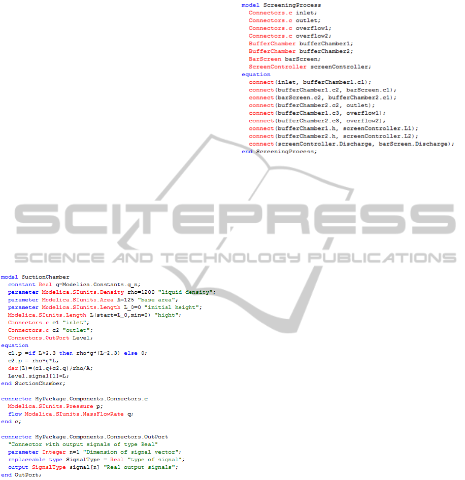
3.1 Screening Process
The screening process may be decomposed to the
following components: two buffering chambers (one
after the inlet and one before the outlet), a Bar
screen crossing between the buffer chambers, and a
screen controller. This is illustrated in Figure 2.
Figure 2: Screening process.
The buffer chamber model has two water
connectors at its base and a third one located at the
overflow level h
of
measured from the chamber’s
base. Another connector of type real output is added
to deliver the liquid height (h) to the screen
controller.
The pressure at the base connectors c
1
and c
2
is
given by:
=
=ℎ
(1)
where is the wastewater density,
g is the
acceleration due to gravity, and ℎ is the wastewater
level in the chamber. The pressure at the overflow
connector c
3
is discontinuous at the threshold height
h
of
(equals 1.6 m in our case) as follows:
=
0, ℎ≤ℎ
ℎ−ℎ
, ℎ>ℎ
(2)
The wastewater level is related to the mass flow
rate in the ports as follows:
ℎ
=
+
+
(3)
where is the cross sectional area of the chamber.
The bar screen is the interface located between
the two buffering champers. The wastewater flow
across this section may be visualized as shown in
Figure 3.
Figure 3: Bar screen visualization.
At a given time, the screen collects an amount of
coarse material causing a friction resistance to the
water flow. This results in a difference in the
wastewater levels across the screen. The waste water
flow has two components; the first one (q
a
) for
which the flow crosses the screen facing
atmospheric pressure (from h
2
to h
1
). The other
remaining component is referred by (q
b
) as
illustrated in Figure 4.
Figure 4: Decomposing the flow across the screen.
The values of these components may be derived
from the Bernoulli equation. Under the assumption
that the screen area is much less than the area of the
inlet buffer base, the following results are obtained:
h
1
h
2
q
a
q
b
c
1
(p
1
,q
1
)
c
2
(p
2
,q
2
)
Inlet
Outlet
Overflow
Overflow
Buffer chamber
Buffer chamber
Bar screen
c
1
(p
1
,q
1
)
c
3
(p
3
,q
3
)
c
2
(p
2
,q
2
)
h
h1
h2
overflow level
overflow level
B
ModelingandSimulationofaWastewaterPumpingPlant
379
=
2
3
2(ℎ
−ℎ
)
⁄
(4)
=
2ℎ
(ℎ
−ℎ
)
⁄
(5)
where is the screen width and is a transparency
coefficient that represents the screen conductivity
ranging between one and zero. At a given time
instant it is related to the amount of the coarse
material accumulated on the screen. Therefore, it is a
function of the total mass flow () across the screen
and a function of the wastewater quality. In analogy
with charging a capacitor, we model as
=
⁄
(6)
where
is a factor that reflects the wastewater
quality. In simulations, we treated it as a constant
equal to 864000, forcing to be about 1 % after
working for five hours at the maximum mass flow
rate.
The total mass flow since =
and the
connectors’ signals are related as follows:
=ℎ
(7)
=ℎ
(8)
=
=
+
(9)
d
d
=
;
(
)
=0
(10)
where (
) is the initial value. When the screen is
triggered by a digital signal (D) to discharge
accumulated coarse material, at =
, is re-
initialized by 0. The bar screen module is
graphically represented as illustrated in Figure 5.
Figure 5: Bar screen icon.
The screen controller senses the amount of
accumulated coarse material by means of the
wastewater levels in the buffer champers. The
controller activates the discharge signal (D)
whenever ℎ
−ℎ
>ℎ
where ℎ
is a preset value
taken 20 cm in the simulations.
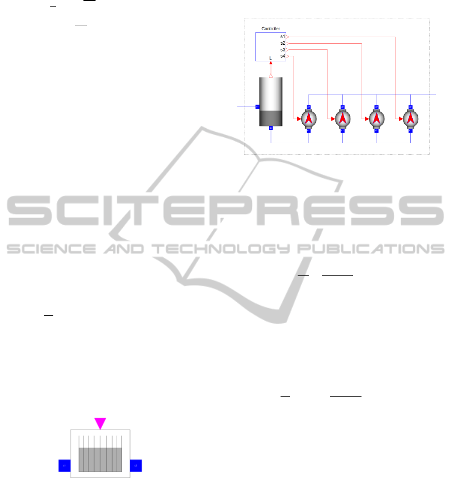
3.2 Pumping Process
This process contains a suction chamber, booster
pumps and a controller as illustrated in Figure 6.
Figure 6: Pumping process.
The suction chamber model is governed by the
following equations:
=
0, ≤2.3
(
−2.3
)
,>2.3
(11)
=
(12)
=
+
(13)
The level signal () is measured relative to the
chamber’s bottom, which is located 2.3 m below the
inlet connector.
A liner head-flow characteristic around the
nominal operating point is used for the booster
pumps (Abdelati et al., 2011) as follows:
=
[
−
−
−ℎ
]
(14)
where a is the slope of the flow-versus-head curve at
the nominal operating point (ℎ
,
), is the
respective pump’s speed, and
is the nominal
speed. The specific data for the installed pumps are:
=8.3//, ℎ
=38,
=360/, and
=1300.
In order to implement the control scheme
specified in Section 2.1, the calculation of the speed
vector, s=(
,
,
,
)
, according to the level
signal (L) is decomposed as shown in Figure 7.
The controller has a PID module with limited
output, anti-windup compensation and set point
weighting (Astrom and Hagglund, 1995). Its output
specifies the required pumping capacity, which has a
minimum of 0 when all pumps are off and a
maximum of 4·1300 when 4 booster pumps run at
their full speed.
c
1
(p
1
,q
1
)
c
2
(p
2
,q
2
)
D
Inlet
Outlet
ICINCO2012-9thInternationalConferenceonInformaticsinControl,AutomationandRobotics
380
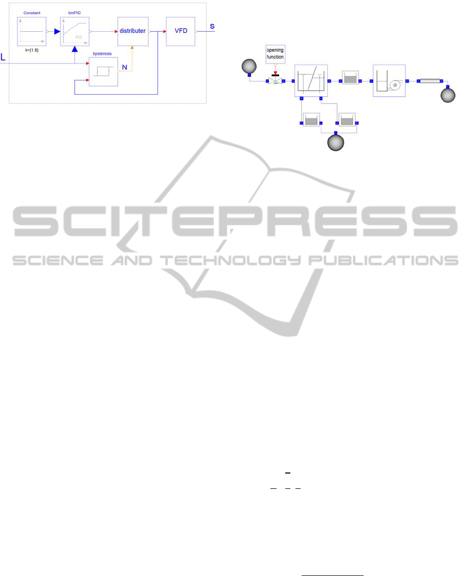
Figure 7: Pumping process controller.
The hysteresis module decides on enabling or
disabling each pump and calculates the number of
enabled pumps (N). The implementation of this
module will be described later. The distributer
divides the PID output value by this number and
assigns the result to the enabled pumps taking into
account that the result has a saturation value of 1300
rpm. The hysteresis module is a sequential circuit
which uses the state of pumps (enabled/disabled),
their assigned speed, and the wastewater level to
calculate their next states. Then it calculates the
number of enabled pumps and delivers it to the
distributer module. The state equation of a pump is
simply the characteristic equation of an RS flip flop
which is set whenever wastewater level exceeds the
set level of the pump and reset whenever the level
drops below the stop level or its speed drops below
its minimum allowed speed. The minimum speed
limits of pumps are 433, 650, 866, and 975 rpm,
respectively. This ensures exempting a pump whose
load share can be carried by the other running
pumps.
The Variable Frequency Drives (VFD) module is
modeled by a first-order block with a time constant
of 5 s resulting in an acceleration time of about half
a minute to move forward or backward between zero
speed and rated speed states.
3.3 Complementary Modules
Encapsulating the screening and pumping processes
into two stand alone modules, the system model will
be as illustrated in Figure 8.
Connectors of the overflow pond and the sink
pond are located above the surfaces of the ponds.
Therefore, they have the atmospheric pressure value
which is our reference (=0). On the other hand,
the connector of the source pond is located at the
bottom of the pond. The wastewater level in the
source pond may vary along the year depending on
the collected sewage. However, the pond is so huge
that its level is safely considered as constant on
weekly or even monthly bases. Consequently, the
pressure at the source pond connector is treated as
constant. This constant is taken as the value found
during the month of June which is about 0.25 bar.
Figure 8: System model.
The gate valve is adjusted manually to control
the daily transmitted wastewater and indirectly
decide on the pumping capacity. If the inlet
wastewater rate exceeds the feasible pumping
capacity, then the automation system should signal a
high level alarm prior to overflow. The operator in
turn, should react immediately by decreasing the
gate valve opening and vice versa. Operator
interaction is expected to be on weakly bases in case
pumping is done all the day. A linear relation
between flow and pressure drop is used for the valve
model. The control signal of the valve is named
and its value ranges from 0 at full closure
to 1 at full opening. The nominal hydraulic
conductance of a valve, , is defined as the ratio of
nominal flow to nominal pressure drop at full
opening. Assuming linear pressure drop, then the
flow is governed by the following equation:
=··(
−
)
(15)
The Bernoulli equation is used to derive the
model of notches. Since they always have inlet
pressure greater than or equal to the corresponding
outlet pressure, their equation reduces to
=
2
2
3
(
−
)
⁄
+
(
−
)
⁄
(16)
where B is the width of the notch.
The transmission pipe is modeled according to
the Hazen-Williams equation (Brater at al., 1996).
The resulting model is
−
=
10.67
.
.
.
.
+
(17)
where is the diameter, is the length, is the
static head, and is the roughness coefficient of the
pipe. This coefficient is about 140 for most pipes as
it does not depend so much on the roughness of the
source
pond
notch
screening process
sink pond
overflow pond
notch notch
pumping process
gate valve
transmission pipe
ModelingandSimulationofaWastewaterPumpingPlant
381
material itself, but on the roughness of the bacterial
slime layer which grows on the pipe wall.
3.4 The Implementation Procedure
This subsection describes briefly how the models
were implemented in Modelica using the Dymola
tool (Dynasim, 2009). The first step was
implementing the liquid connector (c). Its icon is
represented by a small blue square and it is defined
as follows:
connector c
Modelica.SIunits.Pressure p;
flowModelica.SIunits.MassFlowRate q;
end c;
Then, the components necessary to build the top
level module are implemented one by one. For
example, the suction chamber has two liquid
connectors (c1 and c2) in addition to an output
connector (L) of type real. Being governed by Eq.
11, 12, and 13, its Modelica code will be as shown
in Figure 9.
Figure 9: Modelica code of the suction chamber.
Only the equations section along with the
necessary parameters and constants need to be
written by the programmer. The instantiations of
connectors are simply done by dragging-and-
dropping in the graphical interface of Dymola.
Moreover, the tool allows drawing a graphical icon
to represent the component. It also generates code
for graphically interconnected components that build
a higher level module. For example, Figure 10
illustrates the Modelica code that corresponds to the
screening process shown in Figure 2.
Figure 10: Code generated by the graphical tool.
A good modeling methodology starts by
implementing simple models, which can be easily
verified by intuition. It continues with models of
increasing complexity until reaching the top-level
module. At each stage, created components are
connected to form system models whose simulation
results can be compared to expectations from the
mind model. If they agree, the model is verified.
Otherwise, the mathematical model is revised or the
mind model is adjusted through gaining new
physical insight (
Jensen, 2003).
4 SIMULATION RESULTS
The aim of simulations is to validate the consistency
of the derived model and to investigate the behavior
of the system under unfavorable scenarios. Power
failure, excess flow, and operator inattentiveness
may lead to overflow. The implemented control
algorithm is widely used in pumping stations and
claims to minimize the number of restarts of pumps
and the number of running pumps given a desired
daily flow. The running period and the number of
restarts have direct impact on the depreciation of
pumps and their power consumption. Deriving a
formula for the cost function, which also includes
overflow cost and operator satisfaction (utility), is
intended to be done in a future work. The scope of
this paper is to create a working model and simulate
normal and unfavorable running conditions leaving
the evaluation and improvement of the control
algorithm to a complementary work. To this end, the
opening signal of the gate valve and the availability
of electric power are assigned the functions shown
in Figure 11. The opening signal function represents
possible flows along the year. The failure of electric
power supply during the time period [3600 s,
ICINCO2012-9thInternationalConferenceonInformaticsinControl,AutomationandRobotics
382
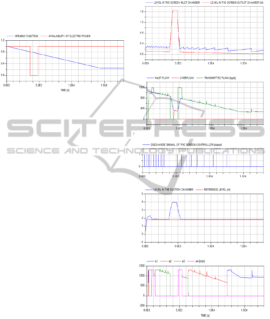
4800 s] is intended to investigate overflow behavior
during a relatively high flow period. The failure is
implemented by suppressing the controllers’ outputs
during the failure period.
Figure 11: Simulation Scenario.
Simulation results which lie within our interest
are shown in Figure 12. As expected, they are
consistent with real world data observed in the plant.
In Figure 12.a, the waste water levels in the screen
chambers are depicted. Shortly after the power
failure, the levels in the chambers reach the level of
the overflow notches (1.6 m) and eventually cause
flood to the overflow pond as shown in Figure 12.b.
In the same figure, the inlet and transmitted flows
are depicted. It is worth to highlight the value of the
outlet flow when the pumps run at their full
capacity. It is about 380, 720, 982, and 1186 kg/s
while the number of pumps equals 1, 2, 3, and 4,
respectively. Figure 12.c illustrates the time
instances when the screen discharge signal is
enabled. This happens whenever the level difference
in the screen chambers reaches 0.2 m. The
wastewater level in the suction chamber is depicted
in Figure 12.d. Apart from the starting and the power
failure periods, the level in the suction chamber is
almost equal to the reference value which is 1.8 m.
The overshoot is expected as it is necessary to
trigger the starting of the pumps. The load share of
these pumps is shown in Figure 12.e. Running
pumps always have equal shares, as desired, and it is
notable that sudden increase in the pump speeds
occurs at screen cleaning instants.
Keeping the wastewater level in the suction
chamber around the reference value implies
adjusting the outlet flow to meet the inlet flow.
However, this does not insure running the plant in
the most efficient way. One should develop a
controller which maximizes a proper performance
measure while keeping the level within allowable
domain. A good performance measure could be the
pumping efficiency which is the ratio of the outlet
flow to the consumed power.
(a)
(b)
(c)
(d)
(e)
Figure 12: Simulation output results.
5 SUMMARY AND OUTLOOK
This work presents an easily manageable model for a
ModelingandSimulationofaWastewaterPumpingPlant
383

wastewater pumping station in northern Gaza. The
resultant model provides a practical tool for
examining the system control under different running
conditions, such as pump failure and changing flow
rates. This simulation model assists in adjusting the
control reference points and parameters to cope with
regular and undesired situations. The simulated
control algorithm is widely used in pumping stations
and it is believed that it works to minimize
maintenance and running costs by minimizing the
number of running pumps and limiting the number of
their restarts for a certain inlet rate.
At the present phase, the ponds of the old
treatment plant serve as a buffer for the wastewater
before being pumped via the NTPS to the new
treatment plant. This buffering stage will not be
available by the completion of the project as the old
plant will be removed and incoming wastewater is
planned to be transmitted directly to the new
treatment plant. Only one small size pond will be left
for collecting emergency overflows at the pumping
station. As a result, the real challenge of the control
problem is not the present phase where a fixed daily
amount of wastewater needed to be transported. In the
final phase, the pump station must handle
instantaneous variation of the wastewater flow.
Accidental overflow will result in an additional re-
pumping cost and undesired environmental
consequences. Therefore, an estimate of the daily
diurnal flow pattern is necessary to examine the plant
controller under daily variation of wastewater flow.
In a future work, we plan to model the daily
diurnal flow pattern and formulate a quantitative
performance measures for running the system. This
will enable us to develop a criterion for optimal
control of pumping stations. We will employ
simulations over long time horizons to respect
special conditions found in Gaza but also many
other developing areas. For example, frequent
failure in the main electric power supply is common
in Gaza city nowadays and requires intensive
operator supervision. Moreover, power produced by
the standby generators is much more expensive than
the power of the main supply. This is a point
normally not considered in deriving the control laws.
Models implementing functions to derive the total
cost of operation similar to models presented in
(Felgner et al., 2011) combined with predictive –
simulation based – hybrid control schemes as in
(Sonntag et al., 2009) are expected to be of great
value under these conditions.
ACKNOWLEDGEMENTS
The authors would like to express their gratitude to
Alexander von Humboldt Foundation for supporting
this work.
REFERENCES
Abdelati, M., Rabah, F., 2007. A Framework for Building
a SCADA System for Beit Lahia Wastewater Pumping
Station, The Islamic University Journal, Natural
Studies and Engineering Series, Vol.15, No. 2, pp
235-245, ISSN 1726-6807.
Abdelati, M., Felgner, F., Frey, G., 2011. Modeling,
simulation and control of a water recovery and
irrigation system, Proceedings of the 8th International
Conference on Informatics in Control, Automation and
Robotics. Noordwijkerhout, The Netherlands.
Astrom, K., Hagglund, T., 1995. PID Controllers: Theory,
Design, and Tuning, North Carolina, Instrument
Society of America, 2nd edition.
Brater, E., King, H., Lindell, J., 1996. Handbook of
Hydraulics, Mc Graw Hill, New York, 7th Edition.
Dynasim AB, 2010. Dymola Dynamic Modeling
Laboratory User Manual. Sweden.
Elmqvist, H., Tummescheit, H., Otter, M., 2003. Object-
Oriented Modeling of Thermo-Fluid Systems,
Proceedings of the 3rd International Modelica
Conference, Linköping.
Felgner, F., Exel, L., Frey, G., 2011. Component-oriented
ORC plant modeling for efficient system design and
profitability prediction. Proceedings of the IEEE/IES
International Conference on Clean Electrical Power
(ICCEP 2011), Ischia , Italy, pp. 196-203.
Jensen, J., 2003. Dynamic Modeling of Thermo-Fluid
Systems with focus on evaporators for refrigeration.
Ph.D. Thesis, Department of Mechanical Engineering,
Technical University of Denmark.
Link K., Steuer H., and Butterlin A., 2009. Deficiencies of
Modelica and its simulation environments for large
fluid systems, Proceedings 7th Modelica Conference,
Como, Italy.
Palestinian Water Authority, 2004. Bidding Documents for
the Construction of Terminal Pumping Station,
NGEST project management unit, Gaza.
Sonntag, C., Kölling, M., Engell, S., 2009. Sensitivity-
based Predictive Control of a Large-scale Supermarket
Refrigeration System. Int. Symp. on Advanced Control
of Chemical Processes (ADCHEM), Istanbul/Turkey,
pp.354-359.
Tiller M., 2004. Introduction to Physical Modeling with
Modelica, Kluwer Academic Publishers.
Massachusetts, 2
nd
Edition.
Werner M. et al., 2006. North Gaza Emergency Sewage
Treatment Plant Project - Environmental Assessment
Study, Engineering and Management Consulting
Center.
ICINCO2012-9thInternationalConferenceonInformaticsinControl,AutomationandRobotics
384
