
Design and Analysis of an Automated Heavy Vehicle Platoon
G´abor R¨od¨onyi
1
, P´eter G´asp´ar
1
, J´ozsef Bokor
1
and L´aszl´o Palkovics
2
1
Systems and Control Laboratory, Computer and Automation Research Institute, Hungarian Academy of Sciences,
Budapest, Hungary
2
Knorr-Bremse Brake-systems Gmbh, Budapest, Hungary
Keywords:
Vehicle Platoon, Peak-to-peak Gain, Model Set Identification, Unfalsification.
Abstract:
From the model set identification through the control design and robust performance analysis to the implemen-
tation and experimental verification, the whole design process for an automated vehicle platoon is presented.
The goal is to demonstrate that safe platooning with acceptable performance can be achieved by utilizing the
services already available on every commercial heavy trucks with automated gearbox. Using the services, the
control design reduces to the selection of four design parameters, the static gain coefficients of the output-
feedback-input-feed-forward controller common for every vehicle. It is experimentally demonstrated, that in
normal driving maneuvers, the spacing errors are less than three meters.
1 INTRODUCTION
Safe control of vehicle platoons requiresstrict guaran-
teed bounds on inter-vehicle spacing errors. In order
to avoid collision the sampled errors are best mea-
sured by its ℓ
∞
norm, so the bounds represent the
worst-case peaks of the spacing errors. Consistent
identification tools are the set membership methods in
the ℓ
1
setting, see e.g. (Gustafsson and M¨akil¨a, 1996;
Milanese and Belforte, 1982; Milanese, 1995). The
identified model sets are employed for on-line model
validation and a priori analysis of the control perfor-
mance measured by the worst-case spacing errors.
Controllers for autonomous vehicle platoons usu-
ally consists of two levels of feedback controllers. At
the lower level a local, vehicle specific controller is re-
sponsible for performing acceleration demands. The
higher level control law is common for all vehicle, it
is designed for satisfying string stability requirements
of the whole platoon. Very short safety gaps can be
guaranteed, under certain constraints on lead vehicle
maneuvers, when detailed engine, gearbox and brake
system models are available, see, e.g., in references
(Nouveliere and Mammar,2007; Gerdes and Hedrick,
1997; Liang et al., 2003). There is, however, some
difficulties in the widespread applicability of these
control methods. The required engine/gearbox/brake
system models are usually not available and not re-
liable for every commercial heavy trucks. Beyond
that, these controllers try to directly excite the brake
cylinder pressures and throttle valve of the engine,
which could also conflict with the existing control
units, such as Electronic Brake System (EBS) and En-
gine Control Unit (ECU).
In this paper the goal is to explore the performance
of an automated vehicle string where, in contrast to
the former solutions, only the standardized and gen-
eral services of the EBS and ECU are used. This
work is an extension of the work that have been pre-
sented in reference (R¨od¨onyi et al., 2012), where the
focus was placed on the analysis of the spacing error
bounds subject to heterogeneity in vehicle dynamics
and inter-vehicle communication failures. Here we
present two model set identification problems, one of
which is an extension of the method introduced in
(Nagamune et al., 1997; Nagamune and Yamamoto,
1998).
In Section 2 the mathematical model of the pla-
toon is presented. The vehicle model set identifica-
tion method is presented in Sections 3 and 4. The
performance of a heterogeneous platoon is analyzed
in Section 5. The experimental results are presented
in Section 6.
Basic notations. The peak norm of a sequence
u(k) is denoted by kuk
∞
=sup
k
|u(k)|, ℓ
∞
denotes
the space of sequences of finite peak norm. The
peak-to-peak norm of a system H is defined by
kHk
1
=sup
u6=0
kHuk
∞
kuk
∞
.
31
Rödönyi G., Gaspár P., Bokor J. and Palkovics L..
Design and Analysis of an Automated Heavy Vehicle Platoon.
DOI: 10.5220/0004009900310037
In Proceedings of the 9th International Conference on Informatics in Control, Automation and Robotics (ICINCO-2012), pages 31-37
ISBN: 978-989-8565-22-8
Copyright
c
2012 SCITEPRESS (Science and Technology Publications, Lda.)

2 STATE-SPACE MODEL OF
VEHICLE PLATOONS
In this section the discrete-time version of platoon
model and controller are briefly summarized.
The longitudinal dynamics of a single vehicle is
approximated by the following first order nominal
model with sampling time T
s
a
i
(k+ 1) = θ
∗
i1
a
i
(k) + θ
∗
i2
u
i
(k), i = 0,1,...,n
where a
i
and u
i
denote the acceleration and accelera-
tion demand of vehicle i, θ
∗
i1
and θ
∗
i2
denote constant
parameters.
The spacing error of the ith follower vehicle is de-
fined by e
i
(k) = x
i
(k) + L
i
− x
i−1
(k) where L
i
denotes
the desired intervehicular space. Without loss in gen-
erality it can be assumed to be zero in the analysis.
The position of the ith vehicle is denoted by x
i
. For
each vehicle, the spacing error dynamics can be writ-
ten as follows
e
i
(k+ 1)
δ
i
(k+ 1)
a
i
(k+ 1)
=
1 T
s
0 0 0
0 1 T
s
−T
s
0
0 0 θ
∗
i1
0 θ
∗
i2
e
i
(k)
δ
i
(k)
a
i
(k)
a
i−1
(k)
u
i
(k)
where δ
i
denote the relative speed of vehicle i and
i− 1. The open-loop model of the whole platoon
x(k+ 1) = A
d
x(k) + B
d
u(k) + E
d
r(k)
is constructed by introducing the state vector x
T
=
[a
0
e
1
δ
1
a
1
··· e
n
δ
n
a
n
], control input vector u
T
=
[u
1
··· u
n
] and reference signal r = u
0
.
The platoon controller is a modified version of
the constant spacing strategy presented in (Swaroop,
1994, Section 3.3.4). The modification resides in
that, instead of measured acceleration, control input
is transmitted through the network. Consequently, the
gear change has lower impact in the control signal
than in the acceleration, so each vehicle can change
gear without deceiving the followers; the vehicles re-
act quicker to maneuver changes; and no need for
filtering the rather noisy acceleration measurements.
The control strategy is defined by the following equa-
tions
u(k) := u
L
(k) + ˆu
N
(k)
u
L
(k) = K
L
x(k)
u
N
(k) = K
N
x(k) + G
N
r(k) + Su(k)
where u
L
contains the locally available radar informa-
tion. Gain matrix K
L
can be constructed based on the
following definition
u
L,1
(k) = −k
1
δ
1
(k) − k
2
e
1
(k)
u
L,i
(k) = −k
1β
δ
i
(k) − k
2β
e
i
(k), i > 1
where i stands for the vehicle index and k
1
:=
q
1
+q
4
+λ+λq
3
1+q
3
, k
2
:=
λ(q
1
+q
4
)
1+q
3
, k
1α
:=
q
4
+λq
3
1+q
3
, k
2α
:=
λq
4
1+q
3
, k
1β
:=
q
1
+λ
1+q
3
and k
2β
:=
λq
1
1+q
3
, where q
1
, q
3
, q
4
and λ are design parameters. Control signal u
N
is con-
structed from the information received from the com-
munication network
u
N,1
(k) = u
0
(k)
u
N,i
(k) =
1
1+ q
3
u
i−1
(k) +
q
3
1+ q
3
u
0
(k)
−k
1α
i
∑
j=0
δ
j
(k) − k
2α
i
∑
j=0
e
j
(k), i > 1
from which K
N
, G
N
and S matrices can be con-
structed.
The communication network has a sampling time
of T = NT
s
and the packet is transmitted after h <
T constant delay. If y(k) denotes the variable to be
transmitted at the network input, then
ˆy(k) =
y(k− h) if
k−h
N
is an integer
ˆy(k− 1) otherwise
denotes the network output at the receiver.
The closed-loop system with the delayed commu-
nication is derived in (R¨od¨onyi et al., 2012). The lo-
cal part u
L
of the controllers run with the faster sam-
pling rate T
s
. By closing the loop with u
L
, re-sampling
with NT
s
, then closing the loop with ˆu
N
and assuming
r(k) = r(k + 1) = ... = r(k + N − 1) we arrive at the
following system
z(k+ N) = A
z
(h)z(k) + E
z
(h)r(k)
A
z
(h) =
A
N
L
+ B
0
(K
N
+ SK
L
) B
1
+ B
0
S
K
N
+ SK
L
S
E
z
(h) =
E
N
+ B
0
G
N
G
N
where the state-space is augmented to
z(k) =
x(k)
u
N
(k− N)
and
B
1
:=
h−1
∑
j=0
A
N−1− j
L
B
L
, B
0
:=
N−1
∑
j=h
A
N−1− j
L
B
L
E
N
:=
N−1
∑
j=0
A
N−1− j
L
E
L
where A
L
= A
d
+ B
d
K
L
, B
L
= B
d
, E
L
= E
d
. The spac-
ing errors can be observed through matrixes C
i
as
e
i
(k) = C
i
z(k), i = 1, 2,...n.
ICINCO2012-9thInternationalConferenceonInformaticsinControl,AutomationandRobotics
32

3 IDENTIFICATION OF MODEL
SETS
Nominal vehicle models and uncertaintysets are iden-
tified in the worst-case ℓ
1
setting. Two circum-
stances motivate the application of this identification
approach. Both the brake system and the drive-line
are functioning as an unknown nonlinear, hybrid sys-
tems with many thousands of program rows organiz-
ing finite state machines. A good description of noise
statistics is not available and only reduced order mod-
els can be considered. It seems to be reasonable to
consider only strict bounds on the disturbances and
unmodelled dynamics. Strict bounds are also useful
in the worst case analysis of spacing error bounds. On
the other hand, these model sets may result in overly
conservative (loose) description of the system. So-
phisticated uncertainty model structures are required
for control performance analysis problems, the elabo-
ration of which is yet left to future work.
In order to obtain a preliminary view of the uncer-
tainty in the vehicle dynamics and actuators including
EBS and ECU softwares, two identification methods
are presented in the section. The first one is an ARX-
type model structure with time-varying parameters.
The basic concept originates in the papers (Nagamune
et al., 1997; Nagamune and Yamamoto, 1998), briefly
presented in the following subsection. Then, these re-
sults are extended in several ways in Section 3.2. In
the second method an OE model structure is identified
in Section 3.4. Both methods are applied for experi-
mental data of a heavy truck in Section 4.
3.1 Identification of Smallest Unfalsified
Sets
Consider the following discrete-time linear single in-
put single output model structure
G(z) =
∑
m
i=1
b
i
z
−i
1+
∑
m
i=1
a
i
z
−i
, θ ∈ P
θ
(θ
∗
,ε)
with time-varying parameter vector θ =
[a
1
,...,a
m
,b
1
,...,b
m
]
T
defined in the cube
P
θ
(θ
∗
,ε
θ
) := {θ : kW(θ
∗
− θ)k
∞
≤ ε}, where the a
priori given diagonal matrix W = diag{
1
ε
θ,1
,...,
1
ε
θ,2m
}
defines the shape of the cube with edges of length
2ε
θ,i
. Given input output data set {u(k),y(k)}
l
k=1
,
the problem is to find the central parameter θ
∗
and
the minimal size ε of the cube such that for every
k = m,...,l there exists a parameter θ ∈ P
θ
(θ
∗
,ε) not
invalidated by the measurements, i.e.
P
θ
(θ
∗
,ε) ∩ D
k
6=
/
0 ∀k = m,..., l
where D
k
:= {θ : y(k) = ϕ
T
(k)θ(k)} and ϕ
T
(k) =
[−y(k−1),...,−y(k− m),u(k−1),...,u(k− m)]. This
problem can be solved by minimizing a convex func-
tion as follows
ε = min
θ
∗
max
m≤k≤l
|y(k) − ϕ
T
(k)θ
∗
|
kW
−1
ϕ(k)k
1
In the following subsection the model structure is
augmented by an additive disturbance term, and the
worst case prediction error is minimized while an op-
timal shape of the parameter cube and a bound for the
disturbance are determined.
3.2 Unfalsified ARX Model Set of
Minimal Prediction Error in ℓ
∞
With the notation of the previous section we can de-
fine the following ARX type model structure, denoted
by M
M = { y(k) = ϕ
T
(k)θ(k) + e(k),
θ(k) ∈ P
θ
(θ
∗
,ε
θ
),
e(k) ∈ P
e
(ε
a
), k = 1,..., l }
where
P
θ
(θ
∗
,ε
θ
) = {θ : kW(θ
∗
− θ)k
∞
≤ 1},
P
e
(ε
a
) = {e : |e| ≤ ε
a
},
ε
θ
= [ε
θ1
,...,ε
θ2m
]
T
,
W = diag
1
ε
θ,1
,...,
1
ε
θ,2m
The shape and size of the uncertainty set char-
acterized by ε
θ
and ε
a
are unknown parameters.
The only information given a priori is the data set
{u(k), y(k)}
l
k=1
.
In order to characterize consistency of the model
set with the data, define hyperplane D
k
in the n+1 di-
mensional extended parameter space of p := [θ
T
e]
T
D
k
:= {p : y(k) = [ϕ
T
(k) e(k)]p}
Let P(θ
∗
,ε
θ
,ε
a
) := {p = [θ
T
e]
T
: θ ∈ P
θ
(θ
∗
,ε
θ
), e ∈
P
e
(ε
a
)} denote the parameter set defining model set
M in the extended parameter space.
Definition 1 (Consistency). The parameter set p ∈
P(θ
∗
,ε
θ
,ε
a
) can reproduce the data if
P(θ
∗
,ε
θ
,ε
a
) ∩ D
k
6=
/
0 ∀k = m,..., l (1)
For given data ϕ(k) and model set parameters θ
∗
,
ε
θ
and ε
a
the output y(k) that the model set can gen-
erate lies between the bounds
¯y(k) = max
θ∈P
θ
(θ
∗
,ε
θ
)
ϕ
T
(k)θ+ ε
a
y(k) = min
θ∈P
θ
(θ
∗
,ε
θ
)
ϕ
T
(k)θ− ε
a
DesignandAnalysisofanAutomatedHeavyVehiclePlatoon
33

With these bounds, the parameter set identification
problem can be formulated as follows.
Problem 1. Assume that we are given a data set
{u(k), y(k)}
l
k=1
. Find a model set characterized by
θ
∗
, ε
θ
and ε
a
such that (1) is satisfied and that mini-
mizes γ :=
1
2
k ¯y(k) − y(k)k
∞
.
3.3 Solution Via Linear Programming
It will be shown that Problem 1 leads to the solution of
a linear programming (LP) problem. In contrast to the
solution of (Nagamune et al., 1997), where for each
D
k
a minimum necessary size parameter ε = ε(D
k
,θ
∗
)
is determined for a given θ
∗
, we characterize consis-
tency with the help of the output bounds
Lemma 3.1. Consistency condition (1) is satisfied if
and only if there exist θ
∗
, ε
θ
and ε
a
such that
y(k) ≤ ϕ
T
(k)θ
∗
+ |ϕ
T
(k)|ε
θ
+ ε
a
, k = m,..., l (2)
y(k) ≥ ϕ
T
(k)θ
∗
− |ϕ
T
(k)|ε
θ
− ε
a
, k = m,..., l (3)
where |.| element-wise takes the absolute value of the
argument.
Proof. We only need to show that
max
θ∈P
θ
(θ
∗
,ε
θ
)
ϕ
T
(k)θ = ϕ
T
(k)θ
∗
+ |ϕ
T
(k)|ε
θ
and
min
θ∈P
θ
(θ
∗
,ε
θ
)
ϕ
T
(k)θ = ϕ
T
(k)θ
∗
− |ϕ
T
(k)|ε
θ
, then
the statement follows from the definitions. The linear
function ϕ
T
(k)θ over a convex polytope takes up its
extreme values at the vertices of the polytope. Let the
vertex set of P
θ
(θ
∗
,ε
θ
) be denoted by V ,
V =
θ : θ = θ
∗
+
±ε
θ,1
.
.
.
±ε
θ,2m
where ± means all combinations. From this the
claims follow.
The following theorem summarizes our results.
Theorem 3.2. The model set M which is consistent
with the data set {u(k), y(k)}
l
k=1
and minimizes γ =
1
2
k ¯y(k) − y(k)k
∞
is the solution of the following LP
problem.
min
θ
∗
,ε
θ
,ε
a
γ
subject to (2), (3) and
γ ≥ |ϕ
T
(k)|ε
θ
+ ε
a
, k = m,...,l
The problem involves 4m + 2 variables and 3(l −
m + 1) inequality constraints, and can be efficiently
solved by rutin CLP in the MPT toolbox for Matlab,
(Kvasnica et al., 2004).
3.4 Identification of OE Models of
Minimal Error in ℓ
∞
In this section an output error model structure is iden-
tified with the smallest error in ℓ
∞
. Suppose, we are
given a data set {u(k),y(k)}
l
k=1
and the model struc-
ture of LTI SISO systems in the form
G(z) =
∑
m
i=1
b
i
z
−i
1+
∑
m
i=1
a
i
z
−i
The set of parameters is divided as θ
a
= [a
1
,...,a
m
]
and θ
b
= [b
1
,...,b
m
]. We are looking for θ
a
and θ
b
that
minimize γ := ky(k)− ˆy(k)k
∞
, where ˆy(z) = G(z)u(z).
This optimization problem is nonlinear in parameter
θ
a
, therefore an nonlinear programming method can
be applied. In case of small noises, good initialization
for θ
a
and determination of the model order can be
attained by using the recent result (Soumelidis et al.,
2011). Once θ
a
is fixed, θ
b
can be computed by linear
programming as follows.
1. Formulate A, B,C, the controllability canonical
state-space representation of G(z). Then C = θ
T
b
.
From this, ˆy(k) = θ
T
b
∑
k−1
j=0
A
k− j−1
Bu( j)
2. Solve the LP problem
min
θ
b
γ
subject to
y(k) − θ
T
b
k−1
∑
j=0
A
k− j−1
Bu( j) ≤ γ, k = m, ...,l
−y(k) + θ
T
b
k−1
∑
j=0
A
k− j−1
Bu( j) ≤ γ, k = m, ...,l
4 MODELLING LONGITUDINAL
VEHICLE DYNAMICS
Several braking experiments have been carried out
with a Volvo FH, 24 tonne three-axle truck. ARX and
OE models of order m = 1 are identified by using the
methods described in the previous section.
4.1 ARX Model Structure
The LP method of Theorem 3.2 was applied to the
model structure
a(k) = a(k− 1)θ
1
(k) + u(k− 1)θ
2
(k) + e(k)
θ(k) := [θ
1
(k) θ
2
(k)]
T
∈ P
θ
(θ
∗
,ε
θ
)
ke(k) − e
∗
k
∞
≤ ε
a
ICINCO2012-9thInternationalConferenceonInformaticsinControl,AutomationandRobotics
34
where a(k) is the longitudinal acceleration computed
by the available onboard computers based on wheel
speed measurements, and u(k) is the acceleration de-
mand defined in an AutoBox connected to the vehi-
cle’s CAN network. An offset error of the measure-
ments can be taken into consideration with parame-
ter e
∗
. The unknown parameters of the model are the
central parameters θ
∗
and e
∗
, and the bounds of the
parameter and noise variation, ε
θ
and ε
a
, respectively.
The one-step ahead prediction of the optimal
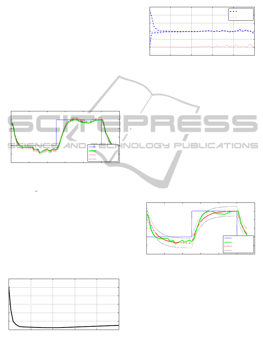
model is plotted in Figure 1. The central parameters
θ
∗
1
and θ
∗
2
correspond to a time constant of 1.13s and
a gain of 9.5 when the model is transformed to con-
tinuous time by zero order hold (T
s
= 0.01). For the
parameter variation we get ε
T
θ
= [0.180.20]1e− 12.
0 2 4 6 8 10 12
−5
−4
−3
−2
−1
0
1
time [s]
acceleration [m/s
2
]
1−step ahead prediction
command
measured
central model
bounds
Figure 1: One step ahead prediction with the central model
with parameter θ
∗
in a braking experiment. Bounds for the
prediction, ¯y and y, are also plotted (thin dotted black lines).
Fixing the maximum allowed noise level ε
a
, the
optimization can be performed in the remaining vari-
ables. Figures 2 and respectively 3 show the depen-
dence of the prediction error bound and the optimal
parameters on the chosen noise levels. It can be seen
that forcing the model set to represent uncertainty by
the time-variation of parameters will result in overly
conservative models. At the optimum, the uncertainty
is described by almost entirely the noise term. We
must conclude that a more sophisticated uncertainty
description is necessary.
0 0.1 0.2 0.3 0.4 0.5
0
1
2
3
4
5
6
Prediction error bound as a function of fixed noise bound
fixed noise bound, ε
a
(minimal γ at ε
a
=0.14282)
Prediction error bound, γ
Figure 2: Worst case prediction error as a function of fixed
noise bound ε
a
in the ARX model structure.
0 0.1 0.2 0.3 0.4 0.5
−0.5
0
0.5
1
1.5
2
2.5
fixed noise bound, ε
a
(minimal γ at ε
a
=0.14282)
Parameters θ
1
and θ
2
Optimal parameter bounds as functions of fixed noise bound
θ
1
bounds
θ
2
bounds
Figure 3: Parameter bounds as functions of fixed noise
bound ε
a
in the ARX model structure.
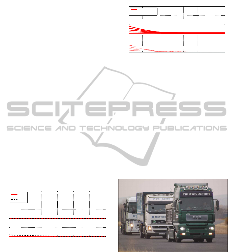
4.2 OE Model Structure
The output-error model structure
a(k) = a(k− 1)θ
1
+ u(k − 1)θ
2
+ e(k) − e(k − 1)θ
1
ke(k) − e
∗
k
∞
≤ ε
a
is identified by applying the LP method presented in
Section 3.4 for identifying θ
2
while θ
1
is determined
by simple line search. The optimal parameters cor-
respond to a time constant of 0.9s and a gain of 1.25
when the model is transformed to continuous time by
zero order hold (T
s
= 0.01). The fit of the model and
the error bounds are plotted in Figure 4. This model
can serve as nominal models in the performance anal-
ysis of the platoon.
0 2 4 6 8 10 12
−5
−4
−3
−2
−1
0
1
time [s]
acceleration [m/s
2
]
Output−error model fit
command
measured
central model
bounds
Figure 4: Fit of the OE model with parameter to the mea-
surements in a braking experiment. Bounds for the error are
also plotted (thin dotted black lines).
5 PERFORMANCE ANALYSIS OF
HETEROGENEOUS PLATOONS
For the case of heterogeneous platoons with nom-
inal LTI models, spacing error bounds in ℓ
∞
are
analyzed.Assume that the allowable reference input
r = u
0
satisfies ku
0
k
∞
≤ u
max
, where u
max
is a given
bound. Then, the worst-case peaks of the spacing er-
rors, as functions of communication delays, can be
DesignandAnalysisofanAutomatedHeavyVehiclePlatoon
35
computed as follows
ε
i
(h) := k e
i
(h,t)k
∞
=
∞
∑
j=0
|C
i
e
A
z
(h)t
E
z
(h)|u
max
In the following numerical analysis ε
i
(h), i = 1,...,n,
are computed when the platoon is not homogeneous
in nominal vehicle parameters θ
∗
i
. It is assumed that
both θ
∗
i,1
and θ
∗
i,2
may differ from vehicle to vehicle
Θ = [θ
∗
1,1
θ
∗
1,2
θ
∗
2,1
θ
∗
2,2
... θ
∗
n,1
θ
∗
n,2
],
θ
∗
i,1
= 1−
T
s
τ
i
θ
∗
i,2
=
T
s
g
i
τ
i
τ
i
∈ {0.6, 0.8}
g
i
∈ {0.9,1.1}
where time constant τ
i
and gain g
i
are parameters of
the continuous-time vehicle models and may take up
their extremal values. It can be shown that the worst-
case platoon configuration is the case when the vehi-
cle model parameters are extremal and alternating in
order. This means that if the platoon is of length n+1,
it is enough to compute ε
i
(h), i = 1,...,n for (n+ 1)
4
systems. Taking the maximum and minimum for the
(n + 1)
4
systems, Figure 5 show the worst case and
best case bounds as functions of the vehicle index i.
The lower bounds are achieved in case of homoge-
neous platoons. For a given set of allowable maneu-
vers, this analysis directly provides hints on choosing
safety gaps between the vehicles in the different con-
trol modes, such as L
i
> ε
i
, assuming zero initial con-
ditions. The analysis is carried out for a range of net-
work delays from h = 0 to h = 8T
s
, but network delay
of this range has negligible impact on the bounds.
1 1.5 2 2.5 3 3.5 4
0
2
4
6
8
10
Vehicle index
Spacing error bound [m]
Peak bounds for spacing errors with different delays
h=0T
s
h=8T
s
Figure 5: Lower and upper bounds on spacing errors, ε
i
for
different network delays. Uncertainty is present in both θ
i1
and θ
i2
. Lower bounds (around zero) correspond to homo-
geneous platoons. Upper bounds at ε
i
= 4 correspond to
platoons of alternating vehicle dynamics.
In the case when gain coefficients are estimated
on-line, for example with the help of parameter adap-
tation methods described in (Swaroop, 1994), acceler-
ation demand can always be scaled so that θ
i2
param-
eters can be set to θ
i2
= 1. Then, spacing errors are
bounded as shown in Figure 6. The bounds reduced
to about one meter.
1 2 3 4 5 6 7 8
0
0.5
1
1.5
2
2.5
h=0T
s
h=0T
s
Vehicle index
Spacing error bound [m]
Peak bounds for spacing errors with different delays
h=8T
s
h=8T
s
upper bounds
lower bounds
Figure 6: Lower and upper bounds on spacing errors, ε
i
for
different network delays. Uncertainty is present only in θ
i1
.
6 EXPERIMENTAL RESULTS
The control strategy presented in Section 2 is imple-
mented on a platoon of three heavy trucks and tested
on a 3km long flight-strip. The leader vehicle, driven
by a driver, is a MAN TGA two-axle tractor of 18
tonne with load cage. The second vehicle is a Volvo
FH 24 tonne three-axle truck. The third one is a Re-
nault Magnum two-axle tractor of 18 tonne with a
semitrailer, See Fig. 7. It is important to remark that
all vehicles are equipped with automatic gear change,
thus acceleration can be attained purely by software.
The communication network consists of radio
transceivers operating on the open 868MHz ISM
narrow-band.
Figure 7: Experimental vehicles in project TruckDAS.
The experimental scenario is started with a ’join-
ing in’ maneuver in which the leader vehicle passes
the others which are travelling at constant speed.
When the last vehicle in the platoon is caught by the
radar of the joining vehicle and its driver enables the
joining maneuver by pressing a deadman-button, the
joining vehicle is accelerated and braked by given
constant values and for sufficient time so that the ve-
hicle arrives approximately at the prescribed distance
ICINCO2012-9thInternationalConferenceonInformaticsinControl,AutomationandRobotics
36
with speed near that of the platoon. After the braking
period the spacing controller is switched on. When
both joining maneuvers are finished, the leader vehi-
cle can accelerate and decelerate and finally stop.
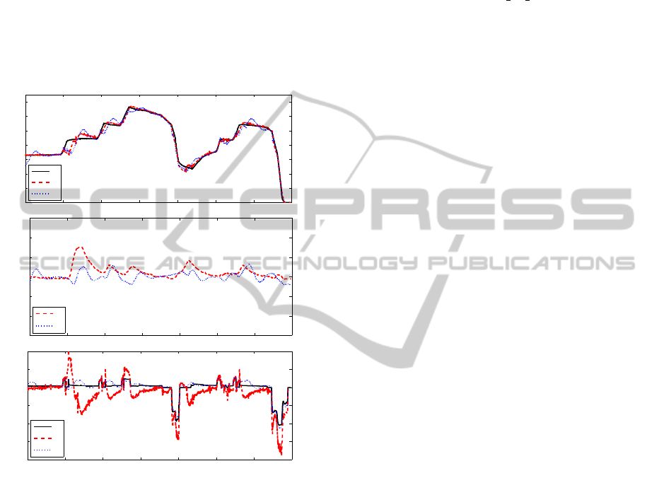
Nine experiments of similar maneuvers were car-
ried out on a 3km long pathway. The maximum spac-
ing error was not greater than 3m during braking, i.e.
in the direction of collision danger. During driving
maneuvers, the maximum leg was not greater than
8m.
0 20 40 60 80 100 120 140
0
10
20
30
40
50
60
70
Communication with both preceding and leader vehicle
speed [km/h]
v
0
v
1
v
2
0 20 40 60 80 100 120 140
−15
−10
−5
0
5
10
15
spacing error [m]
e
1
e
2
0 20 40 60 80 100 120 140
−4
−3
−2
−1
0
1
2
Control signal [m/s
2
]
time [s]
u
0
u
1
u
2
Figure 8: Platoon control experiment.
7 CONCLUSIONS
According to our experiences in a platoon of three ve-
hicles with different types and properties, a safety gap
of 3m can be safe if the following conditions hold:
deceleration of the leader vehicle is not greater than
2m/s
2
and there is some dwell time between inten-
sive acceleration and abrupt braking maneuvers so
that transients can cease.
ACKNOWLEDGEMENTS
This research work has been supported by Control
Engineering Research Group, Hungarian Academy of
Sciences at the Budapest University of Technology
and Economics and the Hungarian National Scien-
tific Research Fund (OTKA) through grant No. CNK-
78168. The research has also been supported by the
Hungarian National Office for Research and Technol-
ogy through the project TECH 08 A2 /2-2008-0088.
REFERENCES
Gerdes, J. and Hedrick, J. (1997). Vehicle speed and spac-
ing control via coordinated throttle and brake actua-
tion. Control Engineering Practice, 5:1607–1614.
Gustafsson, T. K. and M¨akil¨a, P. M. (1996). Modelling of
uncertain systems via linear programming. In Auto-
matica, volume 32. No. 3, pages 319–335.
Kvasnica, M., Grieder, P., and Baoti´c, M. (2004). Multi-
Parametric Toolbox (MPT).
Liang, H., Chong, K. T., No, T. S., and Yi, S. (2003). Vehi-
cle longitudinal brake control using variable param-
eter sliding control. Control Engineering Practice,
11:403–411.
Milanese, M. (1995). Properties of least squares estimates
in set membership identification. In Automatica, vol-
ume 31. No. 2, pages 327–332.
Milanese, M. and Belforte, G. (1982). Estimation theory
and uncertainly intervals evaluation in presence of un-
known but bounded errors: Linear families of models
and estimators. In IEEE Trans. on Automatic Control,
volume AC-27. No. 2, pages 408–414.
Nagamune, R. and Yamamoto, S. (1998). Model set
validation and update for time-varying siso systems.
In Proceedings of the American Control Conference,
Philadelphia, pages 2361–2365.
Nagamune, R., Yamamoto, S., and Kimura, H. (1997).
Identification of the smallest unfalsified model set
with both parametric and unstructured uncertainty.
In Preprints of the 11th IFAC Symposium on Sys-
tem Identification (SYSID97), Kitakyushu, Japan, vol-
ume 1, pages 75–80.
Nouveliere, L. and Mammar, S. (2007). Experimental ve-
hicle longitudinal control using a second order slid-
ing mode technique. Control Engineering Practice,
15:943–954.
R¨od¨onyi, G., G´asp´ar, P., Bokor, J., Aradi, S., Hankovszki,
Z., Kov´acs, R., and Palkovics, L. (2012). Analysis and
experimental verification of faulty network modes in
an autonomous vehicle string. In 20th Mediterranean
Conference on Control and Automation, Barcelona,
Spain.
Soumelidis, A., Schipp, F., and Bokor, J. (2011). Pole
structure estimation from laguerre representations us-
ing hyperbolic metrics on the unit disc. 50th IEEE
Conference on Decision and Control and European
Control Conference (CDC-ECC), Orlando, FL, USA.
Swaroop, D. (1994). String stability of interconnected sys-
tems: An application to platooning in automated high-
way systems. PhD dissertation.
DesignandAnalysisofanAutomatedHeavyVehiclePlatoon
37
