
An Integrated Approach for Efficient Mobile Robot Trajectory
Tracking and Obstacle Avoidance
Aleksandar Cosic, Marko Susic and Dusko Katic
Institute Mihajlo Pupin, Robotics Laboratory, University of Belgrade, Volgina 15, Belgrade, Serbia
Keywords: Mobile Robots, Trajectory Tracking, Obstacle Avoidance, Fuzzy Logic, Intelligent Control.
Abstract: An approach for nonholonomic two-wheeled mobile robot trajectory tracking and obstacle avoiding is
presented in this paper. If the desired trajectory is provided by high level planner, trajectory tracking
problem can be solved in various ways. In this paper, tracking is provided using proportional-integral (PI) or
fuzzy logic controller (FLC). Unfortunately, tracking is never perfect, due to uncertainties and obstacles can
change their positions in time. In order to overcome these difficulties, additional correction controller must
be used. Here is proposed fuzzy controller, which slightly changes control action of the tracking controller
in order to prevent collision with obstacles. This approach is proved to be efficient even in dynamic
environments. Simulation results are presented as illustration of the proposed approach.
1 INTRODUCTION
In recent years, due to growing popularity and
importance of wheeled mobile robots (WMRs) in
many applications, motion control problems
dedicated to WMRs attracted great attention.
Trajectory tracking problem can be considered as a
part of mobile robot navigation problem, which has
been intensively researched, e.g. (Laumond, 1998;
LaValle, 2006; Masehian and Sedighizadeh, 2007).
Considerable research efforts have been made on
trajectory tracking control of two-wheeled
differentially driven mobile robots. Despite the
apparent simplicity of the WMR kinematic model,
the design of stabilizing control law is challenging
due to the existence of nonholonomic constraints.
Varius control strategies have been presented
such as: sliding-mode control, e.g. (Bloch and
Drakunov, 1994), backstepping procedure, e.g.
(Taner and Kyriakopoulos, 2003), dynamic feedback
linearization, e.g. (Oriolo et al., 2002), Lyapunov-
type techniques, e.g. (Mastellone et al., 2008),
adaptive control, e.g. (Fukao et al., 2000), model
predictive control, e.g. (Kühne et al., 2005) and
intelligent techniques, based on neural networks and
fuzzy logic, e.g. (Jiang et al., 2005; Oh et al., 2005).
In general, closed-loop results obtained using
classic control approaches may present undisarable
oscillatory motions. From the other hand, fuzzy
logic may be good option for uncertain systems,
whose behaviour can be described linguistically. In
this paper, two tracking controllers will be designed,
nonlinear PI and fuzzy controller. Unfortunatelly,
due to uncertainties and obstacles movements,
collision with obstacles could happen even if the
high level planner provided collision free path. It is
the reason why additional fuzzy controller must be
introduced, which will correct the control action of
the tracking controller, when mobile robot comes
close enough to the obstacle.
The rest of the paper is organized as follows:
description of the WMR kinematic model is given in
Section 2, design of the control structure in Section
3, simulation results in Section 4, while the
conclusion is given in Section 5.
2 KINEMATIC MODEL OF THE
TWO-WHEELED MOBILE
ROBOT
Schematic model of WMR is shown on Figure 1.
Derivation of the kinematic equations of the two-
wheeled mobile robot is given in (Susic et al., 2011).
World coordinate frame is denoted by {X,O,Y},
while {x
l
,COM,y
l
} denotes local coordinate frame,
attached to the robot, whose origin is placed at the
robot’s centre of mass (COM). State variables are
position and orientation of the robot, i.e. COM
211
Cosic A., Susic M. and Katic D..
An Integrated Approach for Efficient Mobile Robot Trajectory Tracking and Obstacle Avoidance.
DOI: 10.5220/0004010402110216
In Proceedings of the 9th International Conference on Informatics in Control, Automation and Robotics (ICINCO-2012), pages 211-216
ISBN: 978-989-8565-22-8
Copyright
c
2012 SCITEPRESS (Science and Technology Publications, Lda.)
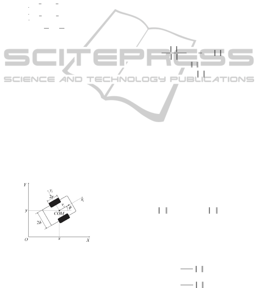
position
and angle between x axes of the
world and local coordinate frame, while ω
L
and ω
D
denote angular velocities of the left and right side
wheels of the robot, respectively, and represent
control inputs, while
denotes COM linear velocity
and
denotes robot angular velocity around COM.
If and denote projections of velocity vector
onto coordinate axis of global coordinate system,
kinematic model of the mobile robot is given by:
cos cos
22
sin sin
22
22
L
D
rr
x
rr
y
rr
bb
(1)
3 DESIGN OF THE CONTROL
SYSTEM
Proposed controller consists of three parts: trajectory
tracking controller (TTC), obstacle avoiding
controller (OAC) and combined controller (CC). It is
assumed that the collision free trajectory is already
provided by high level planner, i.e. virtual vehicle
trajectory is known. TTC provides tracking of the
desired trajectory. For this purpose two controllers
will be presented, nonlinear PI and FLC. PI
controllers are simple and widely used in industrial
practice, while FLCs are intelligent control strategies
which are proved to be efficient in control of
complex systems. Main drawback of FLCs is large
number of parameters which has to be adjusted.
Tracking is never perfect, so, at this point, it is not
ensured that robot will pass from starting to
destination point safely. For this purpose fuzzy OAC
Figure 1: Kinematic model of mobile robot.
is proposed, which generates correction control
signal which moves robot away from the obstacle.
The last part of the control structure is combined
controller. Its role is to combine the control signals
obtained from TTC and OAC into control inputs of
the mobile robot, i.e. to make compromise between
“tracking” and “avoiding” action of the controller.
3.1 Design of the Trajectory Tracking
Controllers
3.1.1 Nonlinear Pi Controller
Tracking controller generates control action which
tries to direct robot to the desired trajectory. Let
denote robot position and orientation,
desired position and orientation at the
same time instant, and
desired velocity Velocity
generated by controller is denoted by
and can be
obtained as:
*
*
00
,
1
,
0,
min , /
v v v
e
e e e
v
e
e
v
zz
pz
z zi z
z
zi
z
Kd
d
T
d
d d d k
(2)
where
is velocity correction, k is positive gain
and d is the dead-zone size, dependent on
.
Tracking error and integral of tracking error are
denoted by
and
, respectively. Proportional gain is denoted by
K
p
, while T
i
stands for integral constant.
Velocity correction is nonlinear function of
errors sum, i.e. dead-zone around desired point is
introduced. Introducing nonlinearity is necessary,
because it does not allow oscillations of robot’s
position near the desired point. Dead-zone size
decreases when desired velocity increases.
Parameter
determines the maximal value of
tracking error near the destination point.
Angular velocities of the motors
are
weighted sums of the linear and angular velocities of
the robot
. So, control generated by controller
is given by:
,
Lt v z z Dt v z z
a a a a
vv
(3)
where
and
denote magnitude and angle of
the velocity vector
given by (2),
approximates derivative of the
, while weights
and
are control parameters. These parameters
weight straight-line and turning capabilities.
Derivative approximation
is given by:
*
,
,
z
z
s
z
z
s
d
T
d
T
e
e
(4)
ICINCO 2012 - 9th International Conference on Informatics in Control, Automation and Robotics
212
where
denotes the sampling time. It can be seen
from (4) that controller tries to align orientations of
the real and virtual robot when they are close
enough, i.e. if their distance is less or equal d.
3.1.2 Fuzzy Logic Controller
Controllers based on fuzzy logic are proved to be
efficient in control of complex systems, where other
control strategies do not provide satisfactory
performance. FLCs try to mimic action of
experienced operator.
Proposed controller is Takagi-Sugeno-Kang
(TSK) type and has three inputs (“distance to virtual
vehicle” - Euclidian distance between real and
virtual COM position, “angle” - angle at which real
robot sees the virtual and “orientation difference” -
difference between virtual and real robot
orientations) and two outputs (“linear velocity” -
linear velocity of the WMR, normalized on [0,1] and
“angular velocity” - angular velocity of the WMR,
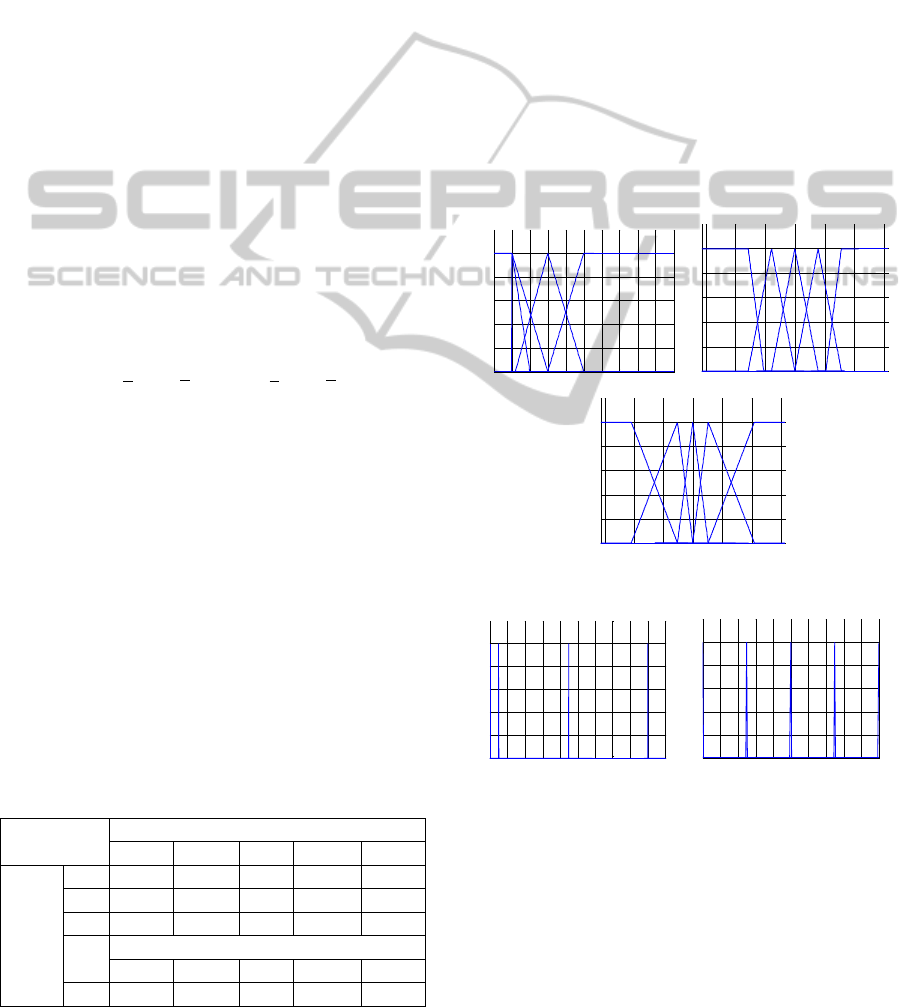
normalized on [-1,+1]). Membership functions of the
linguistic values of inputs and outputs are given on
the Figures 2 and 3.
According to (3), outputs of the whole FLC can
be obtained as:
,
Dt v t t Lt v t t
K v K K v K
(5)
where
and
are normalized linear and angular
velocities produced by the fuzzy inference
mechanism, while
and
are weights which
give the relative importance to straight forward and
turning capabilities.
Fuzzy rule base is given by Table 1. Membership
functions are represented by abbreviations, defined
on Figure 3. Also, every cell is represented by two
linguistic values. The first one corresponds to the
“linear velocity”, while the second one corresponds
to the “angular velocity”. As can be seen from Table
1, there are two sets of fuzzy rules. The first one
takes “distance to virtual vehicle” and “angle” as
inputs. This set of rules is active when robot is not
close enough to the desired point, and controller tries
Table 1: Fuzzy rule base of the TTC.
“angle”
BL
FL
F
FR
BR
“distance to virtual
vehicle”
N
Z/HP
S/Z
S/Z
S/Z
Z/HN
M
Z/FP
M/HP
M/Z
M/HN
Z/FN
F
Z/FP
L/HP
L/Z
L/HN
Z/FN
“orientation difference”
Z/HN
Z/HN
Z/Z
Z/HP
Z/HP
VC
LN
MN
S
MP
LP
to bring the robot close to this point. Second set of
rules takes “distance to virtual vehicle” and
“orientation difference” as inputs. This set of rules is
active when robot comes close enough to the desired
point, trying to align robot’s and desired orientation.
Thus, the idea is to introduce set of rules which
keeps orientation of the real and virtual robot
aligned when they are close enough.
3.2 Design of the Obstacle Avoiding
Controller
Path planning algorithm in complex scenarios with
large number of obstacles might generate path that
guides robot very close to the obstacles. Tracking is
not perfect, so obstacle avoidance is not ensured yet.
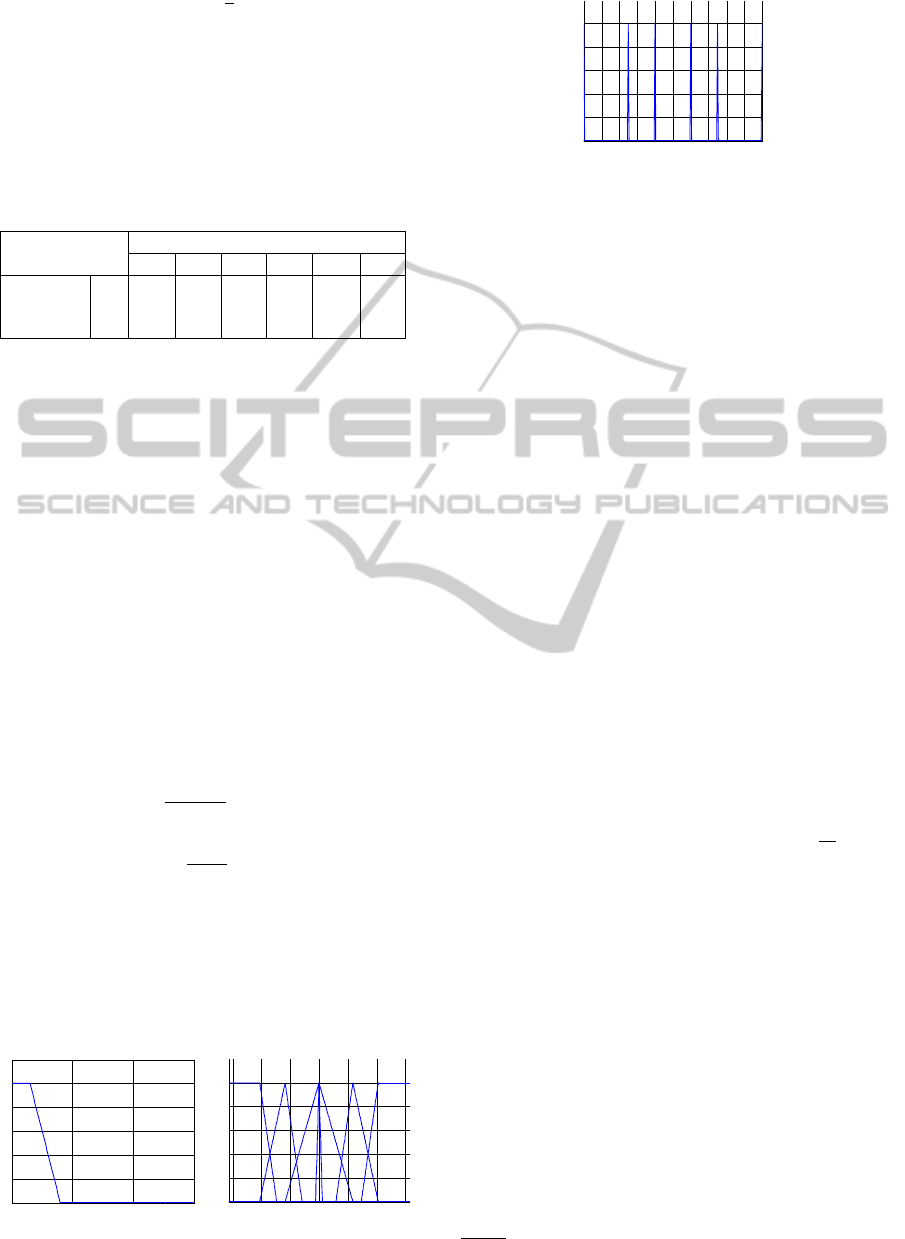
Obstacle avoiding fuzzy controller is two-input
(“distance to obstacle” and “obstacle viewing
angle”) and one-output (“angular velocity
Figure 2: Membership functions of the TTC’s inputs.
Figure 3: Membership functions of the TTC’s outputs.
correction”, normalized on [0,1]) system. Meaning
of the fuzzy inputs and output is similar as in TTC
design. Correction should be generated such that
mobile robot moves away from the obstacle, but
only when it comes close enough to it.
Membership functions of the fuzzy inputs and
output are given on Figures 4 and 5. Output of the
whole OAC is:
0 0.05 0.1 0.15 0.2 0.25 0.3 0.35 0.4 0.45 0.5
0
0.2
0.4
0.6
0.8
1
input variable : "distance to virtual vehicle" [m]
degree of membership
Very
Close(VC)
Near(N)
Medium(M) Far(F)
-3 -2 -1 0 1 2 3
0
0.2
0.4
0.6
0.8
1
input variable : "angle" [rad]
degree of membership
Back Left(BL)
Back Right(BR)
Front
Left(FL)
Front
Right(FR)
Front(F)
-3 -2 -1 0 1 2 3
0
0.2
0.4
0.6
0.8
1
input variable : "orientation difference" [rad]
degree of membership
Large
Negative(LN)
Medium
Negative(MN)
Small(S)
Medium
Positive(MP)
Large
Positive(LP)
0 0.1 0.2 0.3 0.4 0.5 0.6 0.7 0.8 0.9 1
0
0.2
0.4
0.6
0.8
1
output variable : "linear velocity" [rad/s]
degree of membership
Medium(M)
Large(L)
Zero(Z)
Small(S)
-1 -0.8 -0.6 -0.4 -0.2 0 0.2 0.4 0.6 0.8 1
0
0.2
0.4
0.6
0.8
1
output variable : "angular velocity" [rad/s]
degree of membership
Full
Negative(FN) Zero(Z)
Half
Negative(HN)
Full
Positive(FP)
Half
Positive(HP)
An Integrated Approach for Efficient Mobile Robot Trajectory Tracking and Obstacle Avoidance
213
K
(6)
where is output of the fuzzy inference system,
and
is output gain.
Fuzzy rules are given by Table 2. Abbreviations
are also used for membership function
representation. Avoiding action is the strongest
when the obstacle is straight ahead of the robot.
Table 2: Fuzzy rule base of the OAC.
“obstacle viewing angle”
BR
R
FR
FL
L
BL
“distance
to
obstacle”
N
SP
HP
FP
FN
HN
SN
3.3 Design of the Combined Controller
The task of the CC is to combine outputs from the
TTC and OAC in order to obtain control signals of
the mobile robot. It is basically a weighed sum of
TTC and OAC outputs, whose weights depend on
distance between robot and obstacle, i.e. it gives
relative importance to “tracking” and “avoiding”
action. If the robot is close enough to the obstacle,
OAC output becomes dominant, otherwise TTC
output is dominant. Тhe outputs of the CC are given
by:
1 2 1 2
,
L Lt D Dt
K K K K
(7)
where
and
denote the weights, given by (8),
and
are the outputs of the TTC and is
the output of the OAC.
min
min
1
11
max
max
2
22
1
min 1,
max 0,
c
c
K
K d K
d
K
K d K
d
(8)
where d denotes distance between robot and
obstacle,
denotes minimum distance to obstacle
when OAC becomes active,
is the minimum
contribution of the tracking signal in the overall
control, while
is the maximum contribution of
the avoiding in the overall control.
Figure 4: Membership functions of the OAC’s inputs.
Figure 5: Membership functions of the OAC’s output.
4 SIMULATION RESULTS
Proposed algorithm for mobile robot trajectory
tracking is implemented in MATLAB package.
Environment with seven circular obstacles is
adopted. Tracking performance will be presented in
two different scenarios. In the first scenario, planner
knows exact position of the obstacles, so generated
desired trajectory is guaranteed to be collision free.
In further text, this scenario will be denoted by
Scenario I. In the second scenario, some obstacles
slightly changed their positions, while desired
trajectory remained the same (in further text denoted
by Scenario II). Mean-square error (MSE) is adopted
as a measure of tracking quality, and MSE values
obtained in these scenarios are given by Table 3.
It is assumed that robot width is and
wheel radius is . Maximum angular
velocities of the wheels are
. It is assumed that the robot position and
orientation measurements are corrupted with white
Gaussian noise, which standard deviations are 1cm
and 1°, respectively. Starting point is
,
while the destination point is
for the
virtual robot. Starting point and orientation of the
real robot is
.
Results obtained in the Scenario I have been
presented on Figures 6, 7 and 8. Error on the
Figures 6, 7, 9 and 10 is defined as distance between
desired
and robot's position
at the
same time instant. Snapshots of the vehicles on
Figure 8 have been taken at the following time
instants: (0,3,6,10,15,35)s. Virtual robot is
presented by blue dotted line, real robot with PI TTC
controller with red solid line, while the one with
FLC TTC with green solid line. Parameters of all
controllers have been adjusted experimentally. PI
controller parameters are as follows:
.
PI outputs have been filtered with simple first-order
continuous filter whose transfer function is
. Choice of the controller parameters is critical.
0 0.5 1 1.5
0
0.2
0.4
0.6
0.8
1
input variable : "distance to obstacle" [m]
degree of membership
Near(N)
-3 -2 -1 0 1 2 3
0
0.2
0.4
0.6
0.8
1
input variable : "obstacle viewing angle" [rad]
degree of membership
Back
Right(BR) Right(R)
Front
Right(FR)
Front
Left(FL)
Left(L)
Back
Left(BL)
-1 -0.8 -0.6 -0.4 -0.2 0 0.2 0.4 0.6 0.8 1
0
0.2
0.4
0.6
0.8
1
output variable : "angular velocity correction" [rad/s]
degree of membership
Full
Positive(FP)
Half
Positive(HP)
Small
Positive(SP)
Small
Negative(SN)
Half
Negative(HN)
Full
Negative(FN)
ICINCO 2012 - 9th International Conference on Informatics in Control, Automation and Robotics
214
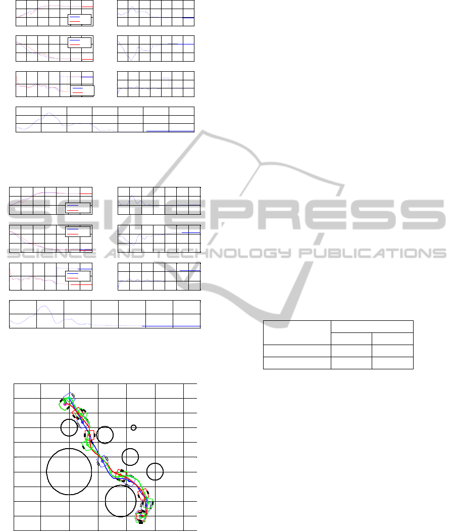
Figure 6: Tracking errors with PI TTC and OAC in
Scenario I.
Figure 7: Tracking errors with FLC TTC and OAC in
Scenario I
Figure 8: Comparative 2D view of robots motion in
Scenario I.
Increase of proportional gain
enhances the
tracking performance, but increases the presence of
noise in control signals. Decrease of
decreases the
tracking error, but may lead to instability.
Parameters
and
weight straight-line and
turning capabilities, so larger value of
is
recommended. Gains of the FLC are also chosen as:
. These parameters weight straight
motion and turning capabilities, respectively, so
larger values of
are advisable, in order to ensure
good tracking in sharp curves.
Output gain of the OAC is adopted as
, while
and
. This
means that the minimal “tracking” contribution is
40%, while maximal “avoiding” contribution is 60%
in overall control action. Critical distance to obstacle
on which CC modifies “tracking” control action with
“avoiding” contribution is
. Figure 8
shows that the “avoiding” contribution degrades the
quality of tracking near the obstacles, but robots
move away from the obstacles, decreasing the risk of
collision. In this case, FLC used as TTC is better
solution.
Results obtained in Scenario II, when obstacles
1, 2, 3 and 6 changed their positions slightly are
shown on Figures 9, 10 and 11. Snapshots of the
vehicles have been taken at the following time
instants: (0,3,7,13,35)s. FLC used as TTC provides
better result again.
Table 3: Mean-square error in different scenarios.
Scenario
MSE value [cm]
PI
FLC
Scenario I
26.9
17.6
Scenario II
51.9
22.7
5 CONCLUSIONS
The solution of trajectory tracking with obstacle
avoiding is presented in this paper. Although it is
assumed that planner which provides collision free
time-parameterized path is available, it is not
necessary. It is enough that only “sketch” of the
trajectory is provided, and OAC will correct control
action and push mobile robot away from the
obstacles. Proposed scheme can be used in different
scenarios with obstacles of arbitrary shape. This
approach can be applied even in dynamic
environments in which exist moving obstacles. The
proposed algorithms will be implemented in real
time control of 4WD mobile robot platform.
0 5 10 15 20 25 30 35
0
2
4
6
x[m]
virtual
real
0 5 10 15 20 25 30 35
-0.5
0
0.5
1
e
x
[m]
0 5 10 15 20 25 30 35
0
2
4
6
y[m]
virtual
real
0 5 10 15 20 25 30 35
-1
-0.5
0
0.5
e
y
[m]
0 5 10 15 20 25 30 35
-5
0
5
[m]
virtual
real
0 5 10 15 20 25 30 35
-5
0
5
10
e
[m]
0 5 10 15 20 25 30 35
0
0.5
1
1.5
tracking error[m]
time[sec]
0 5 10 15 20 25 30 35
0
2
4
6
x[m]
virtual
real
0 5 10 15 20 25 30 35
-0.5
0
0.5
1
e
x
[m]
0 5 10 15 20 25 30 35
0
2
4
6
y[m]
virtual
real
0 5 10 15 20 25 30 35
-1
-0.5
0
0.5
e
y
[m]
0 5 10 15 20 25 30 35
-5
0
5
[m]
virtual
real
0 5 10 15 20 25 30 35
-5
0
5
10
e
[m]
0 5 10 15 20 25 30 35
0
0.5
1
tracking error[m]
time[sec]
1 2 3 4 5 6
0
0.5
1
1.5
2
2.5
3
3.5
4
4.5
5
x[m]
y[m]
1
2
3
4
5
6
7
1
2
3
4
5
6
7
1
2
3
4
5
6
7
1
2
3
4
5
6
7
1
2
3
4
5
6
7
1
2
3
4
5
6
7
An Integrated Approach for Efficient Mobile Robot Trajectory Tracking and Obstacle Avoidance
215
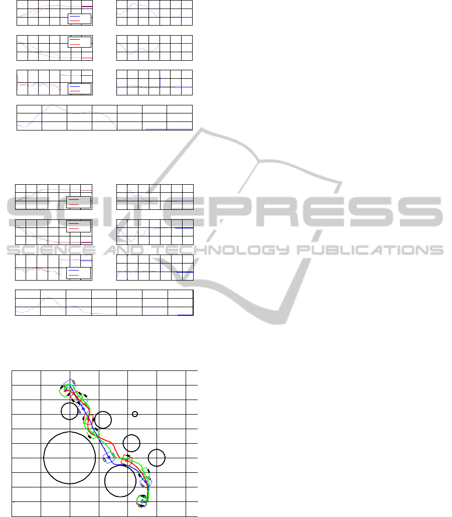
Figure 9: Tracking errors with PI TTC and OAC in
Scenario II.
Figure 10: Tracking errors with FLC TTC and OAC in
Scenario II.
Figure 11: Comparative 2D view of robots motion in
Scenario II.
ACKNOWLEDGEMENTS
The results, presented in the paper, are obtained in
the research projects TR-35003 and III-44008
supported by Ministry of Science of Republic
Serbia.
REFERENCES
Laumond, J., 1998. Robot Motion Planning and Control,
Springer-Verlag, London.
LaValle, S., 2006. Planning Algorithms, Cambridge
University.
Masehian, E., Sedighizadeh, D., 2007. Classic and
Heuristic Approaches in Robot Motion Planning, A
Chronological Review, World Academy of Science,
Engineering and Technology, 29.
Bloch, A., Drakunov, S., 1994. Stabilization of a
Nonholonomic System via Sliding Modes, IEEE
Conference on Decision and Control
Taner, H. G., Kyriakopoulos, K. J., 2003. Backstepping
for Nonsmooth Systems, Automatica, Vol. 39, pp.
1259 – 1265.
Oriolo, G., De Luca, A., Vendittelli, M., 2002. WMR
Control via Dynamic Feedback Linearization:
Decision, Implementation and Experimental
Validation, IEEE Transactions on Control Systems
Technology, Vol. 10, No.6, pp. 835-851.
Mastellone, S., Stipanovic, D., Graunke, C., Intlekofer, K.,
Spong, M., 2008. Formation Control and Collision
Avoidance for Multi-agent Non-holonomic Systems:
Theory and Experiments, The International Journal of
Robotics Research, Vol. 27, No. 1, pp. 107-126.
Fukao, T., Nakagawa, H., Adachi, N., 2000. Adaptive
Tracking Control of a Nonholonomic Mobile Robot,
IEEE Transactions on Robotics and Automation, Vol.
16, pp. 609-615.
Kühne, F., Lages, W. F., Gomes da Silva Jr., J. M., 2005.
Mobile Robot Trajectory Tracking using Model
Predictive Control, 2
nd
IEEE Latin-American Robotics
Symposium
Jiang, X., Motai, Y., Zhu, X., 2005. Predictive Fuzzy
Logic Controller for Trajectory Tracking of a Mobile
Robot, IEEE Mid-Summer Workshop on Soft
Computing in Industrial Applications
Oh, J. S., Park, J. B., Choi, Y. H., 2005. Stable Path
Tracking Control of a Mobile Robot using a Wavelet
Based Fuzzy Neural Network, International Journal of
Control, Automation and Systems, Vol.3, No. 4, pp.
552-563.
Susic, M., Cosic, A., Ribic, A., Katic, D., 2011. An
Approach for Intelligent Mobile Robot Motion
Planning and Trajectory Tracking in Structured Static
Environments, Proceedings of the SISY 2011, pp. 17-
22.
0 5 10 15 20 25 30 35
0
2
4
6
x[m]
virtual
real
0 5 10 15 20 25 30 35
-0.5
0
0.5
1
e
x
[m]
0 5 10 15 20 25 30 35
0
2
4
6
y[m]
virtual
real
0 5 10 15 20 25 30 35
-2
-1
0
1
e
y
[m]
0 5 10 15 20 25 30 35
-5
0
5
[m]
virtual
real
0 5 10 15 20 25 30 35
-5
0
5
10
e
[m]
0 5 10 15 20 25 30 35
0
0.5
1
1.5
tracking error[m]
time[sec]
0 5 10 15 20 25 30 35
0
2
4
6
x[m]
virtual
real
0 5 10 15 20 25 30 35
-0.5
0
0.5
1
e
x
[m]
0 5 10 15 20 25 30 35
0
2
4
6
y[m]
virtual
real
0 5 10 15 20 25 30 35
-1
-0.5
0
0.5
e
y
[m]
0 5 10 15 20 25 30 35
-5
0
5
[m]
virtual
real
0 5 10 15 20 25 30 35
-5
0
5
10
e
[m]
0 5 10 15 20 25 30 35
0
0.5
1
1.5
tracking error[m]
time[sec]
1 2 3 4 5 6
0
0.5
1
1.5
2
2.5
3
3.5
4
4.5
5
x[m]
y[m]
1
2
3
4
5
6
7
1
2
3
4
5
6
7
1
2
3
4
5
6
7
1
2
3
4
5
6
7
1
2
3
4
5
6
7
ICINCO 2012 - 9th International Conference on Informatics in Control, Automation and Robotics
216
