
Predictive Data Reduction in Wireless Sensor Networks using Selective
Filtering
David James McCorrie
1
, Elena Gaura
1
, Keith Burnham
2
and Nigel Poole
1
1
Cogent Computing ARC, Coventry University, Priory Street, Coventry CV1 5FB, U.K.
2
Control Theory and Applications Centre, Coventry University, Priory Street, Coventry CV1 5FB, U.K.
Keywords:
Signal Reconstruction, Optimization Problems in Signal Processing, Change Detection Problems Instrumen-
tation Networks and Software.
Abstract:
In a wireless sensor network, transmissions consume a large portion of a node’s energy budget. Data reduction
is generally acknowledged as an effective means to reduce the number of network transmissions, thereby
increasing the overall network lifetime. This paper builds on the Spanish Inquisition Protocol, to further reduce
transmissions in a single-hop wireless sensor system aimed at a gas turbine engine exhaust gas temperature
(EGT) monitoring application. A new method for selective filtering of sensed data based on state identification
has been devised for accurate state predictions. Low transmission rates are achieved even when significant
temperature step changes occur. A simulator was implemented to generate flight temperature profiles similar to
those encountered in real-life, which enabled tuning and evaluation of the algorithm. The results, summarized
over 280 simulated flights of variable duration (from approximately 58 minutes to 14 hours) show an average
reduction in the number of transmissions by 95%, 99.8% and 91% in the take-off, cruise and landing phases
respectively, compared to transmissions encountered by a sense-and-send system sampling at the same rate.
The algorithm generates an average error of 0.11 ± 0.04 °C over a 927 °C range.
1 INTRODUCTION
Research into the use of wireless instrumentation
in the aerospace industry is growing, both within
academia and industry. In the UK alone several large
projects are currently reporting positively on wireless
sensor network (WSN) based developments for this
sector (Mitchell et al., 2011), (Pinto et al., 2010).
Generically, wireless measurement is considered
an attractive option particularly for aircraft engines.
It could reduce the complexity, weight, and cost of
engine monitoring as well as provide increased sen-
sor density, higher data rates, and enhanced sen-
sor deployment flexibility (Yedavalli and Belapurkar,
2011).
Whilst in-flight engine monitoring and control
based on WSN is a long term aim, in the short-to-
medium term, the use of wireless instrumentation is
envisaged mainly for engine design and test environ-
ments.
The research the authors have engaged with is to-
wards in-flight engine monitoring. It aims to create
Highly Efficient Autonomous Thermocouple (HEAT)
system prototypes for EGT monitoring. A primary
goal is to deliver robust, long lived wireless thermo-
couple systems which sample at rates of over 1 Hz.
The drive towards long lived, low power wireless sys-
tems is essential to the domain, given that nodes need
to run until the next service of the engine to avoid dis-
ruption of operation and need to be powered by exist-
ing energy harvesting technology (Adnan and Harb,
2011).
The HEAT hardware system developed, is com-
posed of multiple battery powered thermocouple sen-
sor nodes, located around the circumference of an en-
gine casing. Each sensor node can sample at 1 Hz
- 5 Hz from a Type-K thermocouple and reports the
EGT data back to the sink node. Nodes use the
CC2530 low powered ZigBee radio from Texas In-
struments (TI) and a MAX6675 cold junction com-
pensation chip. The nodes support Low Power Sleep.
When a HEAT sensor node’s power consumption
was analysed, it was found that a transmission of a
single sample accounts for 75 % of the total consump-
tion, whilst sleeping and sensing account for 24 % and
1 % of the consumption, respectively. Reducing the
number of transmissions will thus provide consider-
able savings in power consumption and increase the
165
James McCorrie D., Gaura E., Burnham K. and Poole N..
Predictive Data Reduction in Wireless Sensor Networks using Selective Filtering.
DOI: 10.5220/0004010601650170
In Proceedings of the 9th International Conference on Informatics in Control, Automation and Robotics (ICINCO-2012), pages 165-170
ISBN: 978-989-8565-21-1
Copyright
c
2012 SCITEPRESS (Science and Technology Publications, Lda.)

network lifetime.
The contribution brought by this paper consists
on a method for drastically reducing transmissions
in EGT wireless sensing systems. The work builds
on previous research in the area of dual predic-
tion schemes (DPSs) for wireless sensor systems.
In particular, we propose an application bespoke
state prediction and selective filtering method to be
used in conjunction with Spanish Inquisition Proto-
col (SIP) (Goldsmith and Brusey, 2010) (described
in Section 4). The proposed method is generically
suitable for applications where the data stream ex-
hibits a combination of steady states and significant
step changes. The performance of the algorithm de-
veloped is tightly correlated with the absolute values
of the sensor readings. Thus in order to tune and eval-
uate its performance an EGT simulator was also de-
veloped.
The remainder of this paper is structured as fol-
lows, Section 2 briefly describes related work in the
area of data reduction for wireless sensor systems.
Section 3 describes the simulator used to evaluate the
proposed algorithm. Section 4 considers the SIP as
the fundamental the data reduction method within the
HEAT system. Section 5 presents the selective filter-
ing (SF) algorithm integrated with SIP. Results are
given in Section 6, and concluding remarks are pre-
sented in Section 7.
2 RELATED WORK
Whist it is important to reduce the number of trans-
missions in a wireless networked system, it is equally
important to accurately capture the phenomena being
monitored. For the application at hand, transmissions
reductions through sampling rate reduction can not be
considered; HEAT nodes need to ensure sampling at
least at 1 Hz. Data compression and reduction is how-
ever an alternative approach to long lived networks
with specified requirements for data quality.
Many methods for data compression and reduc-
tion within a WSN have been proposed. Dictionary
based compression algorithms such as Lossless En-
tropy Compression (LEC) (Marcelloni and Vecchio,
2009) provide a byte reduction on a per packet ba-
sis, although would require sensor readings to be
buffered in order to reduce the number of transmis-
sions. Schoellhammer et al. (2004) model the sensor
readings using a liner model, by buffering the read-
ings until the residual error of a liner fit exceeds a
predefined error threshold. Due to the real-time re-
quirement of the HEAT system, buffering approaches
are not applicable.
The class of DPS algorithms solve the problem of
having to buffer sensor readings. By using a model on
the sensor node and the sink node, new readings can
be predicted without having to transmit further data.
When the error between the models exceeds a toler-
able threshold, new model parameters are transmit-
ted. Large reductions in the the numbers of transmis-
sions can be accomplished using the DPS approach,
while keeping a real-time knowledge of the system’s
state (Anastasi et al., 2009). A variety of implemen-
tations exist for the approach described above. Jain et
al. (2004) use a Dual Kalman Filter (DKF) as the sys-
tem model. Santini and Römer (2006) use an Least
Mean-Square (LMS) filter. Le Borgne et al. (2007)
present a general method for adaptively selecting the
model using a statistical procedure termed racing.
Such a method allows the most optimal model, from
a discrete set of models stored on the sensor node, to
be learned over time. Although considerable trans-
mission reductions are reported for a variety of case
studies, none of these approaches respond well to step
changes in the sensed data. (A summary of the re-
sults of these algorithms can be found in (Goldsmith
and Brusey, 2010) and (Borgne et al., 2007).) These
works have, however inspired the authors here to-
wards the reported developments.
3 EGT SIMULATOR
The EGT simulator attempts to produce flight like
data to be used in evaluating the proposed algorithms.
The simulator consists of an EGT phenomena model
(PM) and a thermocouple sensor model (SM), as
shown in Figure 1. For the purpose of this paper, the
output from the PM, denoted s, is considered as the
actual EGT. The output from the SM is taken to be
the thermocouple readings, denoted y.
Flight profiles are split into three main phases:
take-off, cruise and landing. At the start of the flight
the EGT is relatively low. During take-off, the EGT
rises sharply to around 1000 °C where it remains
fairly constant for the majority of the flight. During
the final landing phase, the EGT decreases to ambi-
ent temperature, with some oscillation to replicate ob-
served practice.
For the purpose of this simulation study, the take-
off and landing sequences, shown in Table 1, are con-
sidered to be consistent. The cruise sections of the
flight are of variable duration, denoted d, which is
regarded as an input to the simulator. To simulate
a typical cruise phase of the flight, a nominal EGT
of 830 °C is chosen. Furthermore, to accommodate
different altitudes and weather conditions, a uniform
ICINCO2012-9thInternationalConferenceonInformaticsinControl,AutomationandRobotics
166

Noise
Flight
profile
Smooth
profile
EGT model
Sensor
model
s
(actual
EGT)
y
(sensor
reading)
d
(cruise
duration)
Take-off
& landing
sequences
smoothing
factor
Noise
Std Dev.
Simulator
Figure 1: Simulator architecture.
distribution of the EGT about the nominal value of
±30 °C is randomly selected at the start of each cruise
section. Over the course of the cruise phase, there are
additional adjustments to the flight pattern, at random
times during every 90-120 minutes, i.e. in a uniformly
distributed random manner. These transients consist
of an increase in EGT by 25 °C for 60 seconds, fol-
lowed by a further cruise section and the cycle repeats
until the cruise phase is complete.
Table 1: Flight sequence for take-off and landing phases,
which is identical in every simulated flight.
Phase EGT (
◦
C) Duration (s)
Start engine 400 40
410 5
390 30
Taxi 430 220
Manoeuvring 390 5
394 7
390 4
394 8
395 3
Take off 950 10
900 430
920 10
Pull back 880 224
High idle 500 200
Landing 463 10
442 5
459 7
441 4
465 8
Reverse thrust 750 15
Engine off 20 30
Once the flight profile sequences have been gener-
ated, smoothing is applied to provide a gradual transi-
tion between flight phases. This facilitates a realistic
EGT of the engine between the various steady state
sections. To realise this, an exponentially weighted
moving average (EWMA) filter with a value for the
smoothing factor, denoted α, of 0.4 is applied to the
generated time series.
It is believed that the standard deviation of the
sensor noise at cruise temperature is around 0.52 °C.
Consequently, Gaussian noise, with a standard devia-
tion of 0.52 °C, is added to the PM output to simulate
realistic thermocouple data.
4 SPANISH INQUISITION
PROTOCOL
The Spanish Inquisition Protocol is a generic data
reduction algorithm developed by Goldsmith and
Brusey, designed to reduce the number of transmis-
sions in a WSN (Goldsmith and Brusey, 2010). The
underlying principle is that transmissions should only
be made when sensor readings are not as expected, i.e.
when some pre-defined change threshold is violated.
By using a model of the system, sensor readings can
be reconstructed at the sink node within a defined er-
ror tolerance.
A model state vector, denoted X
t
, is calculated on
the sensor node and shared with the sink. This state
vector is used on both the sensor and sink to predict
the future system state at every time step. As the
predicted state, denoted X
0
t
, diverges from the actual
measured state, so the reconstruction error, defined as
ε =
|
X
0
t
− X
t
|
, increases. When this error exceeds a de-
fined threshold, a new model state vector is calculated
and shared.
The data reduction that SIP provides is dependent
on model quality and the calculation of the predicted
state, denoted X
0
t
. In this paper a piecewise linear
model is used, as demonstrated in (Goldsmith and
Brusey, 2010). The model state vector is defined as
X
t
= (x
t
, ∆x
t
)
T
. Where x
t
denotes the predicted value
and ∆x
t
denotes the predicted rate of change. It is
then possible to predict future states between trans-
missions using,
X
0
t
=
1 t
0 1
X
t
5 SIGNAL ESTIMATION USING
SELECTIVE FILTERING
The more accurate the predicted rate of change, the
longer the state prediction will remain within the al-
lowable error range. Hence, the more predictable the
signal the greater the reduction in transmissions. It is
important, therefore, to remove as much noise from
the signal as possible, which is done by filtering the
data. Selective filtering (SF) is a rule based method
of selecting between multiple filters in real time, each
optimised for a different part of the signal. The sig-
nal is modelled as a sequence of states and transitions.
PredictiveDataReductioninWirelessSensorNetworksusingSelectiveFiltering
167
State transitions are identified by a predefined set of
rules specific to the application. Each state has it’s
own filter, selected from a bank of filters and it’s own
predictor, which estimates the rate of change. Two
states are defined in this application, steady and vari-
able, shown in Figure 2.
Variable
State
Steady State
Steady State
Figure 2: System states within the flight profile.
Steady states are defined as periods of low rate of
change, and is the initial system state. The expected
value x
t
is found by filtering the sensor sample x
t
with
an EWMA filter having a value for α of 0.01. A tran-
sition to variable state is identified when a sample x
t
deviates from x
t
by more than a specified threshold,
denoted b, so that
|
x
t
− x
t
|
> b. For this application,
an appropriate value for the breakout threshold b was
found to be 1.6 °C.
A variable state is defined as a period of large
rates of change in the data. During this state a sec-
ond filter can be used, or as in this application, sam-
ples can remain unfiltered. A moving window, de-
noted W , of the n most recent samples is stored. A
steady state resumes when the range of values in the
window is less than a given threshold, r, such that
max(W ) − min(W ) < r.
Accurate state prediction depends on the calcula-
tion of the two components in the SIP model state
vector. These are: the predicted value, denoted x
t
and
and the predicted rate of change, denoted ∆x
t
. The SF
method improves the quality of the prediction by re-
ducing signal noise. When the rate of change is accu-
rate, the model will take longer to diverge from the ac-
tual sensor readings, resulting in fewer transmissions.
In the steady state ∆x
t
is calculated using the origi-
nal SIP method, ∆x
t
=
x
t
−x
l
t
, where l is the time of last
transmission. Recognising that the rates of change in
the variable and steady states are different, improve-
ment can be gained by reinitialising the model state
vector on each state change. In a steady state, there
is, by definition, little change in the temperature. The
best estimate of the initial ∆x
t
was found to be 0.
When transitioning from a steady to a variable
state, the initial expected value is defined as x
c
= x
c
,
where c denotes the time of the transition to the vari-
able state. Here the expected rate of change is cal-
culated as ∆
x
c
=
x
c
−x
l
c−l
, where x
l
is the last expected
value from the preceding steady state at time l, and x
c
is the sensor reading at the time of transitioning. Sub-
sequent predicted values are calculated as x
t
= x
t
and
rate of change using ∆x
t
= x
t
− x
t−1
.
Moreover, since a variable state starts with a large
change in temperature followed by a convergence to
a steady state, it can be assumed that there is a high
probability that future ∆x
t
will be smaller than ∆x
t−1
.
Based on this assumption, it is postulated that ∆x
t
can
be better predicted with ∆x
t
= γ(x
t
− x
t−1
) where γ ∈
(0, 1]. Where γ determines the strength of the bias of
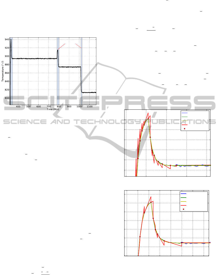
the rate of change towards a steady state. Figure 3
shows the reconstructed signal before and after bias.
320 330 340 350 360
Tim e (Min)
890
900
910
920
930
940
Tem perat ure (
o
C)
noise
filtered
signal
reconstruct ed
transm ission
(a) Before bias
320 325 330 335 34 0 345 350 355
Tim e (Min)
880
890
900
910
920
930
940
950
Tem perat ure (
o
C)
noise
filt ered
signal
reconstruct ed
transm ission
(b) After bias
Figure 3: More accurate rate of change estimation after bias.
6 RESULTS
Using the simulator described in Section 3, a compari-
ICINCO2012-9thInternationalConferenceonInformaticsinControl,AutomationandRobotics
168
son is made between the performances of the Kalman
filter, the EWMA filter, and the SF, as described in
Section 5, when applied to the simulated EGT data.
In particular it is of interest to assess their ability to
filter the data, as well as the impact on the number of
transmissions when they are used in conjunction with
SIP.
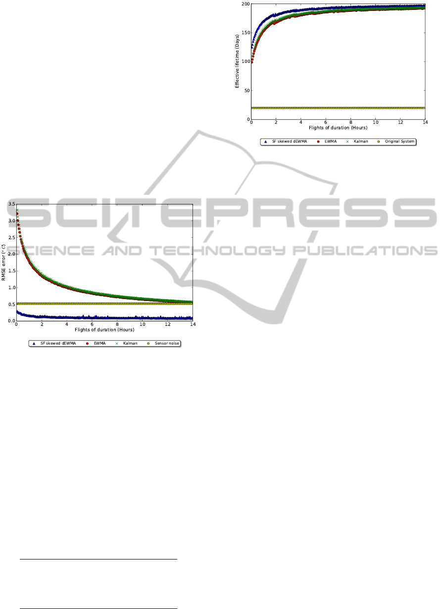
SF reduces the noise while preserving the under-
lying signal, as observed by the reduction of the root
mean squared error (RMSE) between the filtered and
noise free signal, while the EWMA and Kalman filters
increased the RMSE. In order to provide a fair com-
parison in further tests, the EWMA and Kalman filters
were tuned to have a maximum error from the original
signal of 3.5 °C. The simulations were run again with
the new filter parameters and resulting RMSE can be
seen in Figure 4.
Figure 4: RMSE error between the original signal and the
filtered value.
Using an error threshold of 0.5 °C, 280 random
flights are generated with cruise lengths from 0 to 13
hours at 3 minute intervals, Table 2 shows the percent-
age number of samples that would need to be trans-
mitted per hour for each algorithm. Figure 5 shows
the expected battery lifetime of a node running each
algorithm. It is important to note that the expected
lifetime shown is the relative effective lifetime. As-
suming the aircraft continuously serviced flights of
the given duration, d. Each flight immediately fol-
lowing the previous flight, this would be the expected
number of days the HEAT node is expected to last.
Table 2: Mean percentage of samples transmitted per hour
in each phase of a flight.
Samples transmitted per Hour (%)
Filter Take off Cruise Landing
EWMA 7.9 0.4 16.4
Kalman 7.5 0.3 14.8
SF 4.8 0.2 9.5
Figure 5: Comparing expected battery lifetime when using
different data reduction methods.
7 CONCLUSIONS
It has been found that the new SF algorithm, compris-
ing of SIP and SF, when applied to the HEAT sys-
tem has considerably increased the battery lifetime of
a sensor node. The new SF approach has be found
to reduce the sensor error, as well as the overall sys-
tem error. It is expected that the method could be
adapted to other steady state systems with significant
step changes in signal values.
There are some assumptions that have been made
during the evaluation of this work, which may affect
performance in a real deployment. The simulation as-
sumes normally distributed noise, with a fixed stan-
dard deviation. However, in reality this may not be
the case, and the system parameters may change over
time. If this is the case then the breakout threshold
values would need to be adjusted accordingly. Such
an observation would lead naturally to an adaptive
breakout threshold in response to the varying param-
eters.
A further assumption is that the temperature in the
steady state is constant, i.e. no variation; in reality one
could expect there would be some variation.
The encouraging results presented in this paper
provide an opportunity for further exploration. For
example, the algorithm presented uses a linear model
and it is considered that further reductions in trans-
mission is possible if a non-linear model were to be
used.
ACKNOWLEDGEMENTS
The Authors acknowledge the support of Meggitt
(UK) Limited, Basingstoke, UK; TRW Conekt, Soli-
hull, UK and EPSRC.
PredictiveDataReductioninWirelessSensorNetworksusingSelectiveFiltering
169

REFERENCES
Adnan and Harb (2011). Energy Harvesting: State-of-the-
art. Renewable Energy, 36(10):2641–2654.
Anastasi, G., Conti, M., Francesco, M. D., and Passarella,
A. (2009). Energy conservation in wireless sensor net-
works: A survey. Ad Hoc Networks, 7(3):537–568.
Borgne, Y.-A. L., Santini, S., and Bontempi, G. (2007).
Adaptive model selection for time series prediction
in wireless sensor networks. Signal Processing,
87(12):3010–3020.
Goldsmith, D. and Brusey, J. (2010). The Spanish Inqui-
sition Protocol—model based transmission reduction
for wireless sensor networks. In Sensors, 2010 IEEE,
pages 2043–2048.
Jain, A., Chang, E. Y., and Wang, Y. F. (2004). Adap-
tive stream resource management using Kalman fil-
ters. In Proceedings of the 2004 ACM SIGMOD in-
ternational conference on Management of data, pages
11–22. ACM.
Marcelloni, F. and Vecchio, M. (2009). An efficient loss-
less compression algorithm for tiny nodes of monitor-
ing wireless sensor networks. The Computer Journal,
52(8):969–987.
Mitchell, J., Dai, X., Sasloglou, K., Atkinson, R., Strong, J.,
Panella, I., Cai, L., Mingding, H., Wei, A., Glover, I.,
et al. (2011). Wireless communication networks for
gas turbine engine testing. International Journal of
Distributed Sensor Networks.
Pinto, J., Lewis, G. M., Lord, J. A., Lewis, R. A., and
Wright, B. H. (2010). Wireless data transmission
within an aircraft environment. In Antennas and Prop-
agation (EuCAP), 2010 Proceedings of the Fourth Eu-
ropean Conference on, pages 1–5.
Santini, S. and Romer, K. (2006). An adaptive strategy for
quality-based data reduction in wireless sensor net-
works. In Proceedings of the 3rd International Con-
ference on Networked Sensing Systems (INSS 2006),
pages 29–36.
Schoellhammer, T., Greenstein, B., Osterweil, E., Wim-
brow, M., and Estrin, D. (2004). Lightweight temporal
compression of microclimate datasets. In Conference
on Local Computer Networks, pages 516–524.
Yedavalli, R. and Belapurkar, R. (2011). Application of
wireless sensor networks to aircraft control and health
management systems. Journal of Control Theory and
Applications, 9:28–33.
ICINCO2012-9thInternationalConferenceonInformaticsinControl,AutomationandRobotics
170
