
Mechatronic System Optimization based on Surrogate Models
Application to an Electric Vehicle
Moncef Hammadi, Jean-Yves Choley, Olivia Penas and Alain Riviere
LISMMA, SUPMECA-PARIS, 3 Rue Fernand Hainaut, 93400 Saint-Ouen, France
Keywords:
Mechatronic Design, Optimization, Surrogate Models, Modelica, Electric Vehicle.
Abstract:
Preliminary optimization of mechatronic systems is an extremely important step in the development process of
multi-disciplinary products. However, long computing time in optimization based on multi-domain modelling
tools need to be reduced. Surrogate model technique comes up as a solution for decreasing time computing in
multi-disciplinary optimization. In this paper, an electric vehicle has been optimized by combining Modelica
modelling language with surrogate model technique. Modelica has been used to model the electric vehicle
and surrogate model technique has been used to optimize the electric motor and the transmission gear ratio.
Results show that combining surrogate model technique with Modelica reduces significantly computing time
without much decrease in accuracy.
1 INTRODUCTION
Mechatronic Systems (MS) are interdisciplinary
products with a synergistic spatial and functional in-
tegration of mechanical, electronic and software sub-
systems (Craig, 2009).
The great challenge in mechatronic design lies in
optimizing a complete system with various physical
phenomena related to interacting heterogeneous sub-
systems.
Several multi-domain modelling tools such as
Bond-Graphs, VHDL-AMS, Matlab/Simulink and
Modelica are used for preliminary design of MS.
For instance, Modelica (Elmqvist et al., 1998)
combines object-oriented concepts with multi-port
methods for modelling and simulation of physical
systems. It includes a declarative mathematical de-
scription of models and provides a graphical mod-
elling approach. Multi-domain model library of
lumped parameter elements can be created and added
to the default Modelica library for future use. The
end results of Modelica modelling is a system of
differential-algebraic equations (DAE) that represents
the complete mechatronic system. So that, Modelica
is considered as an ideal tool for preliminary design
of MS. However, optimizing a mechatronic system
based on DAE is computationally expensive, due to
the considerable number of simulation evaluations.
For this reason, substituting DAE system with sur-
rogate models, using statistical methods, is one way
of alleviating this burden. The polynomial Response
Surface Method (RSM) (Box and Wilson, 1951) is
commonly considered as the first surrogate modelling
technique. It uses a polynomial formulation to ap-
proximate anexact function. Other techniques such as
Kriging (Krige, 1951) and Artificial Neural Networks
(ANNs) of Radial Basis Functions (RBF) (Hardy,
1971), (Hopfield, 1982) and (Powel, 1985) are also
used to model complex relationships between inputs
and outputs. Surrogate models are also known as
metamodels (Blanning, 1975).
In this paper, both RMS and ANNs of RBF sur-
rogate models have been generated from a Modelica
model of an Electric Vehicle (EV). After their val-
idation and comparison of their accuracy, the ANN
of RBF surrogate model has been chosen to optimize
the electric motor and the gear ratio of the EV. The
optimization based on the surrogate model has been
comparedwith an optimization based on the Modelica
model. Results found are compared with a real case of
an electric vehicle developed by general motors(GM
EV1). Results show an interesting reduction in com-
puting time of optimization without significantly af-
fecting the accuracy.
2 SURROGATE MODELLING
RSM and ANNs of RBF have been used in this study
due to their high accuracy and ease of use. The prin-
11
Hammadi M., Choley J., Penas O. and Riviere A..
Mechatronic System Optimization based on Surrogate Models - Application to an Electric Vehicle.
DOI: 10.5220/0004011900110016
In Proceedings of the 2nd International Conference on Simulation and Modeling Methodologies, Technologies and Applications (SIMULTECH-2012),
pages 11-16
ISBN: 978-989-8565-20-4
Copyright
c
2012 SCITEPRESS (Science and Technology Publications, Lda.)
cipal features of these two surrogate modelling tech-
niques are described in the following section.
2.1 Response Surface Method
As it has been mentioned, RSM uses a polynomial
formulation to approximate an exact function or a
simulation process F(X); where X is the input design
vector that can be represented by a matrix as:
X =
x
11
x
12
... x
1n
x
21
x
22
... x
2n
... ... ... ...
x
m1
x
m2
... x
mn
(1)
n and m are the number of design variables and the
number of sample points, respectively.
The approximation function F
a
(X) is therefore ex-
pressed as:
F
a
(X) = a+
n
∑
i=1
b
i
x
i
+
n
∑
i=1
c
i
x
2
i
+
n−1
∑
i=1
n
∑
j=i+1
d
ij
x
i
x
j
+ ...
(2)
Polynomial degree in RSM models is frequently less
than or equal to 2. Coefficients a, b
i
,c
i
,d
ij
,... are es-
timated by means of the least squares method.
2.2 Artificial Neural Network of Radial
Basis Functions Method
In an ANN of RBF, a response F(X) is approximated
with F
a
(X) as a linear combination of radial basis
functions Φ
j
.
F
a
(X) =
m
∑
j=1
ω
j
.Φ
j
(kX− µ
j
k) (3)
µ
j
are the centres of the radial functions and ω
j
are
the weighting coefficients that can be determined by
the least squares method.
2.3 Validating a Surrogate Model
The surrogate model F
a
(X) and the approximated
function F(X) are related as follows:
F
a
(X) = F(X) + E (4)
The validation of the surrogate model is performed
through the evaluation of the residual vector E. This
evaluation can be made by calculating several quanti-
ties such as the mean error (Em), the root mean square
error (Erms) and the maximum error (Emax), which
are respectively expressed as:
Em
i
=
|
m
∑
j=1
(F(x
ji
) − F
a
(x
ji
))|
m
; 1 ≤ i ≤ n (5)
Erms
i
=
s
m
∑
j=1
[F(x
ji
) − F
a
(x
ji
)]
2
m
; 1 ≤ i ≤ n (6)
Emax
i
= max
j
(|F(x
ji
)−F
a
(x
ji
)|); 1 ≤ i ≤ n;1 ≤ j ≤ m;
(7)
3 APPLICATION: ELECTRIC
VEHICLE OPTIMIZATION
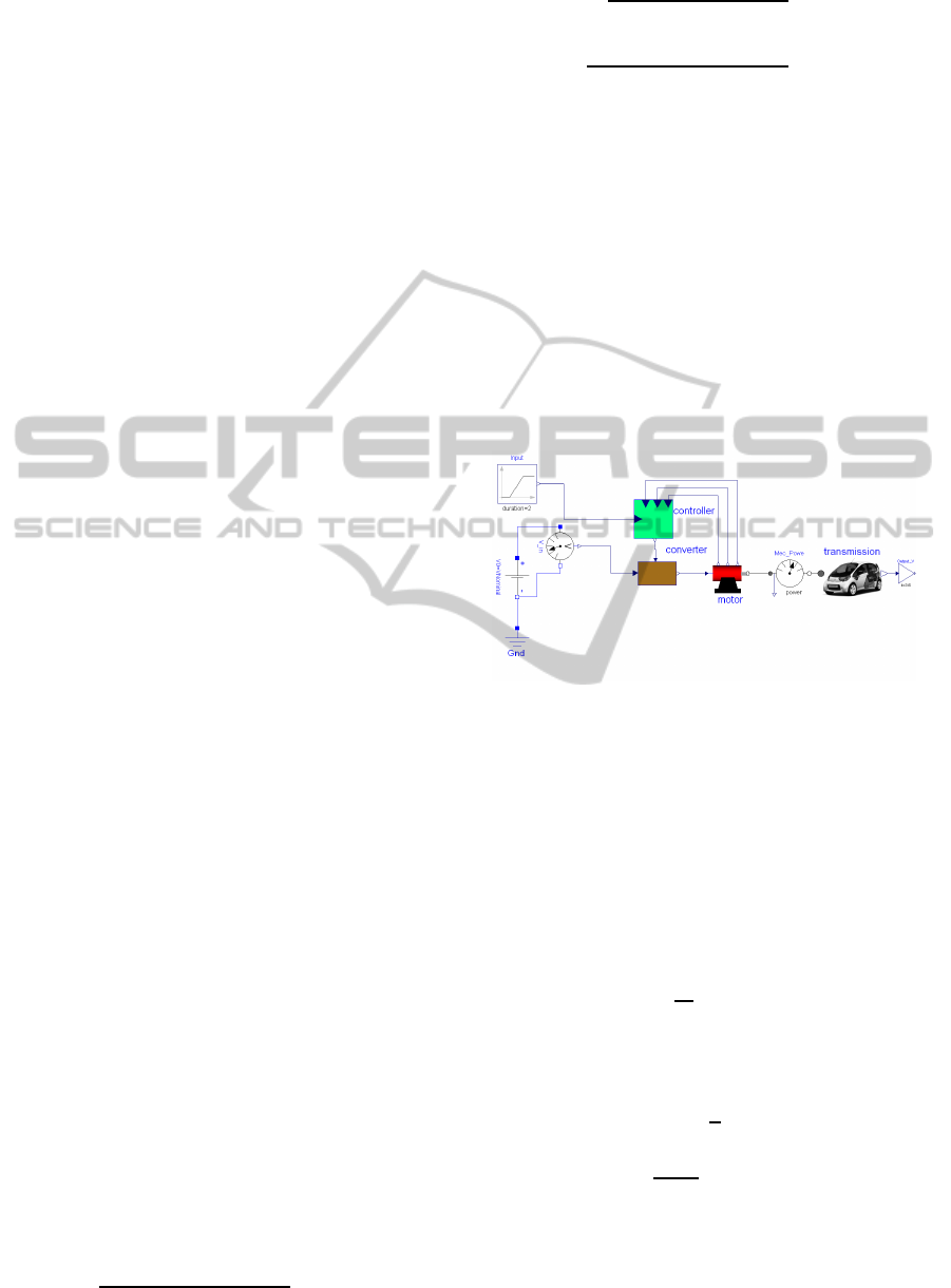
Figure 1 shows EV model which has been performed
using Modelica language. The EV is composed of a
battery (312 V), a power converter, a controller, an
electric motor and a transmission. The objective of
Battery
Accelerator pedal
Meca. Power sensor
Velocity output
w
i
v
Figure 1: Electric vehicle model (Modelica).
this study is to optimize the maximum electric power
Pe
Max
of the motor and the overall transmission gear
ratio G
r
. This optimization should respect a perfor-
mance constraint of acceleration to reach a velocity
V
10
= 100 km/h in 10 seconds. The electric motor is
modelled by the following equations (parameters and
variables are described in Tables 1 and 2).
k.ω
m
= V
emf
(8)
T
m
= k.i (9)
V
e
= L.
di
dt
+ R.i+V
emf
(10)
P
e
= V
e
.i (11)
The transmission model is defined by:
F
t
= M.g. f
r
+
1
2
.d
air
.C
D
.A
f
.v
2
+(M + I.
G
2
r
η
g
.r
2
).a+ M.g.sin(α)
(12)
P
m
= F
t
.v (13)
For the purpose of comparing the simulation results
with a real case, we chose values that match the elec-
tric vehicle EV1 of General Motors (GM), which are
SIMULTECH2012-2ndInternationalConferenceonSimulationandModelingMethodologies,Technologiesand
Applications
12
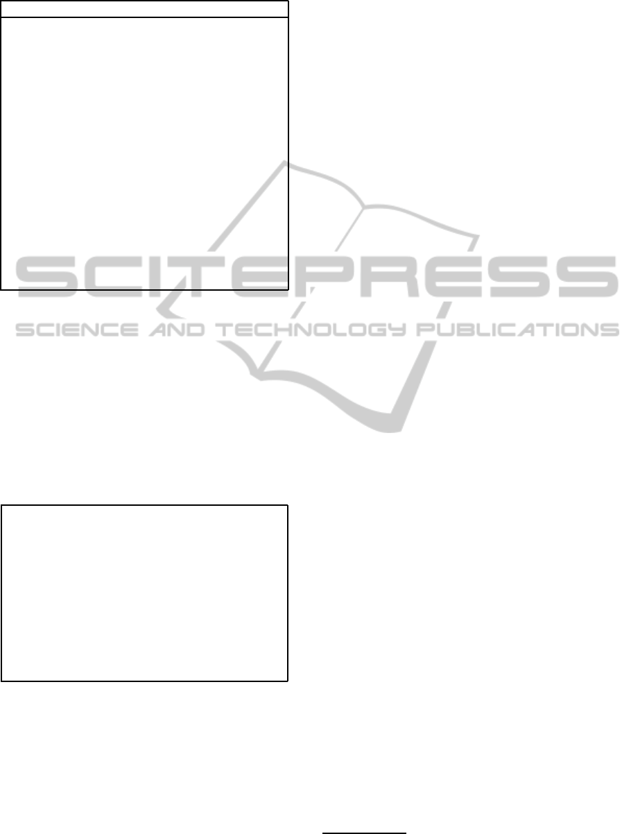
Table 1: Electric vehicle parameters.
parameter value
Vehicle mass M(kg) 1540
Gravity acceleration g(m/s) 9.81
Coefficient of rolling resistance f
r
0.0048
Density of the air d
air
(kg/m
3
) 1.205
Drag coefficientC
D
0.19
Frontal area A
f
(m
2
) 1.8
Moment of inertia of the motor I(kg.m
2
) 0.03
Radius of the tyre r(m) 0.3
Slope angle α(rad) 0
Motor characteristics k(N.m/A) 0.2
Motor internal resistance R(Ω) 0.02
Motor inductance L(H) 0.01
Gear system efficiency η
g
0.95
Gear ratio G
r
opt.
Motor maximum power Pe
Max
(W) opt.
Motor maximum speed ω
M
(rad/s) const.
Motor critical speed ω
C
(rad/s) const.
published in (Larminie and Lowry, 2003). These pa-
rameters are given in Table 1. As indicated in Table 1,
the maximum electric power Pe
Max
and the gear ratio
of the system connecting the motor to the axle G
r
are
to be optimized. The maximum motor speed ω
M
and
the critical speed ω
C
are defined as constraints. ω
C
is the minimum speed above which the electric motor
powers the transmission efficiently. Table 2 gives the
variables which are dependant of time during simula-
tion. We introduce an optimizing objective variable
Table 2: Electric vehicle variables.
Motor rotational speed ω(rad/s)
Electromotive forces V
emf
(V)
Motor torque T
m
(N.m)
Electric current in motor i(A)
Voltage input V
e
(V)
Tractive effort F
t
(N)
Vehicle velocity v(m/s)
Vehicle acceleration a(m/s
2
)
Electric motor instant power P
e
(W)
Mechanical power P
m
(W)
Velocity at 10 seconds V
10
(km/h) ≈ 100km/h
V
10
(km/h) that represents the vehicle velocity at 10
seconds. The goal is to reach 100km/h. In the accel-
eration test, the controller and the power converter act
to power the electric motor with current in order to
provide a torque T
m
defined as:
T
m
= p
a
.Pe
max
/ω
C
(if ω ≤ ω
C
)
T
m
= p
a
.Pe
max
/ω
M
(if ω ≥ ω
M
)
T
m
= p
a
.Pe
max
/ω else
(14)
The percentage of acceleration (p
a
), during the accel-
eration test, reaches 100% in 2 seconds.
Based on the precedent mathematical formulation,
a Modelica model of the EV has been elaborated to be
simulated on an intervaltime of 30 seconds. The input
design vector X for the surrogate models is defined as:
X = [G
r
,Pe
Max
,ω
c
,ω
M
] (15)
The output variable is defined by V
10
which is deter-
mined by the Modelica simulations at every input de-
sign point.
The design space limits for X are defined by : 2 ≤
G
r
≤ 13; 90000 ≤ Pe
Max
≤ 110000; 600 ≤ ω
C
≤ 900;
1000 ≤ ω
C
≤ 1400.
The sample points of the design space domain
havebeen determined using the Design of Experiment
(DoE) technique with a Latin Hypercube method
(Mackay et al., 1979).
Automatic evaluation of the output variable has
been performed using iSIGHT software
1
, which has
been also used to elaborate both RSM and ANN of
RBF surrogate models.
The formulation of the optimization problem is de-
fined as follows:
min Pe
Max
, for 90000 ≤ Pe
Max
≤ 110000
min G
r
, for 2 ≤ G
r
≤ 13
max V
10
, for 98 ≤ V
10
≤ 101
1100 ≤ ω
M
≤ 1400
600 ≤ ω
C
≤ 900
(16)
To solve the non-linear multi-objective optimizing
problem, a sequential quadratic programming algo-
rithm called Non-Linear Programming by Quadratic
Lagrangian (NLPQL) (Schittkowski, 1985) has been
used. NLPQL is well suited for non-linear problems
with few objectives and continuous design space.
4 RESULTS AND DISCUSSION
In this paper, we have combined Modelica modelling
technique with surrogate model method for modelling
and optimization of an electric vehicle. Both RSM
and ANN of RBF surrogate models have been elabo-
rated.
Table 3 gives the evaluation of residual vector E
for both RSM and ANN of RBF models.
Results show that ANN of RBF surrogate model
presents a better accuracy than RSM model. Figure
2 shows the distribution of residuals for the both sur-
rogate models. The results of validation prove the ca-
1
http://www.simulia.com/products/isight.html
MechatronicSystemOptimizationbasedonSurrogateModels
-ApplicationtoanElectricVehicle
13
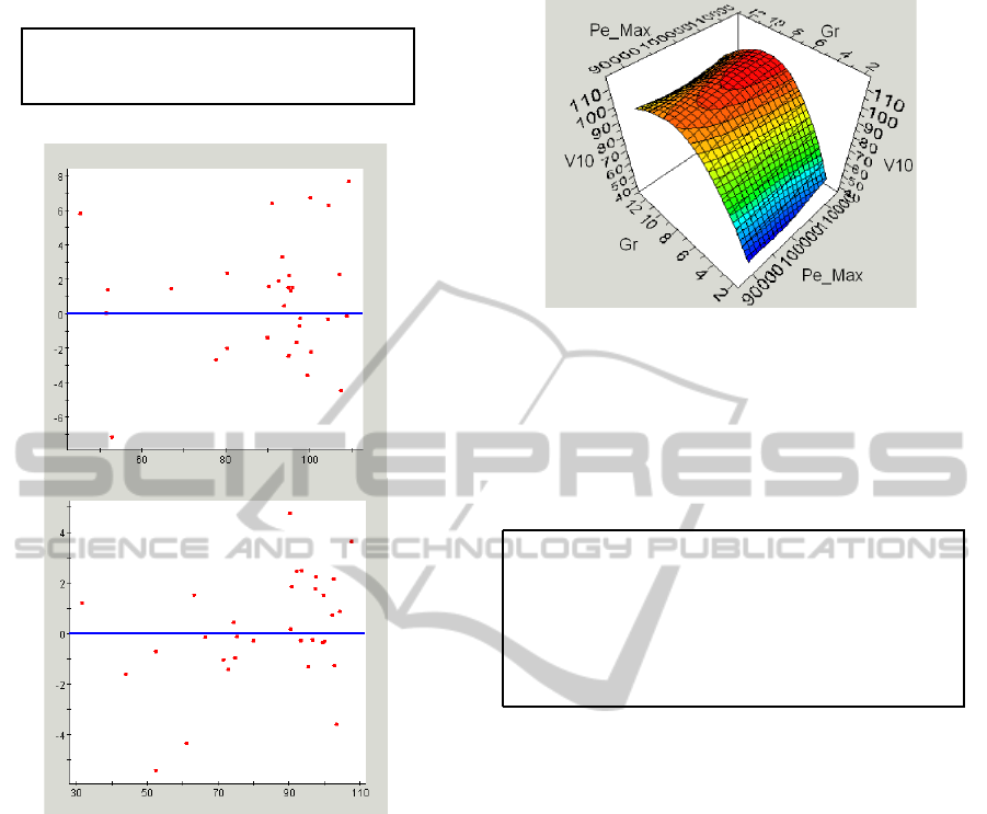
Table 3: Residuals in RMS and RBF models.
Em (%) Erms (%) Emax (%)
RSM 4.1 5.4 11.9
RBF 2.1 2.8 7.1
actual
actual
residual
residual
RMS
RBF
Figure 2: Residual distribution of surrogate models (RSM
and RBF).
pacity of RBF models to approximate non linear re-
sponses. However, RSM model is simpler and eas-
ier to exchange between modelling platforms. In our
case, the algebraic model elaborated for the RSM sur-
rogate model is:
V
10
= − 81.29+ 19.G
r
+ 0.002.Pe
max
− 0.0847.ω
c
+ 0.0383.ω
M
− 1.1942.G
2
r
+ 0.007.G
r
.ω
c
+ 0.0003.G
r
.ω
M
(17)
Such simple mathematical model is useful for system
engineers at high abstraction level for system analysis
and decision making.
A response surface (V
10
= F(G
r
,Pe
Max
)) for the
RBF surrogate model is given by Figure 3. This re-
sponse surface shows that V
10
reaches a maximum,
which justifies the need to optimize V
10
.
Table 4 shows results of optimization based on
Figure 3: Response surface for ANN of RBF surrogate
model: V
10
= F(G
r
,Pe
Max
).
ANN of RBF surrogate model and a comparison
with an optimization based on the Modelica model.
Results show a good agreement between the two op-
Table 4: Optimization results.
RBF Modelica Err.(%)
Gr 9.15 10.1 9.4
Pe
Max
(kW) 102 98 5.2
V
10
(km/h) 99 100.7 1.7
ω
C
(rad/s) 828 780 6.1
ω
M
(rad/s) 1112 1154 3.6
Computing time(s) 4 332
timizations with an important gain of computing time
for the optimization based on the ANN of RBF surro-
gate model (4 seconds for RBF surrogate model and
332 seconds for Modelica model).
These results are close to those published for the
electric vehicle GM EV1. Indeed, for EV1 the electric
motor has a power Pe
Max
= 100kW, maximum speed
of 12000 rpm(ω
M
= 1256 rad/s), ω
C
= 600 rad/s
and a transmission gear ratio G
r
= 11 (Larminie and
Lowry, 2003). The choice of G
r
affects the perfor-
mance of acceleration but also has an influence on
other requirements such as the maximum vehicle ve-
locity, which has not been consideredin this optimiza-
tion. This explains the little difference between values
of G
r
found by optimization and the value chosen by
GM for EV1.
To verify the performance constraint of acceler-
ation test with the case of EV1 vehicle, we have
fixed the following values in the Modelica model:
Pe
Max
= 100kW; ω
C
= 600rad/s; ω
M
= 1256rad/s
and G
r
= 11.
Figure 4 shows the input signal of pedal accelera-
tion and the output vehicle velocity. This figure con-
firms that the electric vehicle reaches a velocity of 100
km/h in 10 seconds.
SIMULTECH2012-2ndInternationalConferenceonSimulationandModelingMethodologies,Technologiesand
Applications
14
0 5 10 15 20 25 30
-10
0
10
20
30
40
50
60
70
80
90
100
110
120
130
Time [s]
Input signal of acceleration (%)
V(km/h)
V(km/h)
Figure 4: Results of Modelica simulation during an acceler-
ation test of the EV (accelerator signal and vehicle velocity).
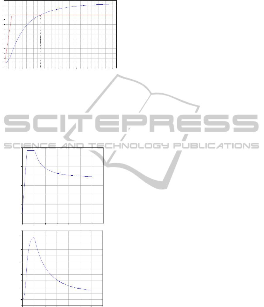
Figure 5 shows the variation of the electric current
and power during the performance test of accelera-
tion. The electric current reaches a maximum of 330
A and the electric power reaches a maximum of 98
kW. The value of the maximum current helps in the
choice of the battery. The simulation near the opti-
0 10 20 30
0E0
2E4
4E4
6E4
8E4
1E5
0 10 20 30
-50
0
50
100
150
200
250
300
350
Electric current i(A)
Electric power (W)
Time (s)
Time (s)
Figure 5: Electric current (top) and electric power (bottom)
during acceleration test of the EV.
mal solution is performed to verify the output design
variables. To improve the optimization accuracy, it
is possible to perform a second optimization on the
Modelica Model, but near the optimal solutions given
by the optimization based on the surrogate models. In
this case, surrogate models play a role of assistant in
optimization. This alternative has longer time of com-
puting but with a better precision, and in most cases
time will be shorter than direct optimization on Mod-
elica model without knowing the neighbourhoods of
the optimal solution.
5 CONCLUSIONS
An electric vehicle has been modelled using Model-
ica language. This model has been used as a support
to develop ANN of RBF and RSM surrogate mod-
els. A comparison of accuracy of the two surrogate
models has been made. It confirms that ANN of RBF
method is more accurate that RSM in the case of elec-
tric vehicle modelling. ANN of RBF surrogate model
has been used to optimize the electric motor and the
gear ratio of the EV. Results show the important gain
in computing time compared to direct optimization
based on the Modelica model, without affecting a lot
accuracy. Results of simulation in the case of acceler-
ation test have been compared to a real case of an EV
(GM EV1), and results show a good agreement with
those published.
Thus, combining Modelica and surrogate mod-
elling techniques is an effective method to reduce
design time and minimize complexity of optimizing
mechatronic systems.
REFERENCES
Blanning, R. (1975). The construction and implementation
of metamodels. Simulation, 24(6):177184.
Box, G. E. P. and Wilson, K. B. (1951). On the experi-
mental attainment of optimum conditions (with dis-
cussion). Journal of the Royal Statistical Society, Se-
ries B, 13:1–45.
Craig, K. (2009). Mechatronic system design. Technical
report, ASME Newsletter.
Elmqvist, H., Mattsson, S., and Otter, M. (1998). Modelica
: The new object-oriented modeling language. In The
12th European Simulation Multiconference, Manch-
ester, UK.
Hardy, R. L. (1971). Multiquadratic equations of topology
and other irregular surfaces. Journal of Geophysical
Research, 76:1905–1915.
Hopfield, J. (1982). Neural networks and physical sys-
tems with emergent collective computational abilities.
Proc. Natl. Acad. Sci., 79:2554–2558.
Krige, D. (1951). A statistical approach to some basic mine
valuation problems on the witwatersrand. Journal
of the Chemical, Metallurgical and Mining Society,
52:119–139.
MechatronicSystemOptimizationbasedonSurrogateModels
-ApplicationtoanElectricVehicle
15

Larminie, J. and Lowry, J. (2003). Electric Vehicle Technol-
ogy Explained. John Wiley & Sons.
Mackay, M. D., Beckman, R. J., and Conover, W. J. (1979).
A comparison of three methods for selecting values of
input variables in the analysis of output from a com-
puter code. Technometrics, 21:239–245.
Powel, M. (1985). Radial basis functions for multi-variable
interpolation: A review. In IMA Conference on Algo-
rithms for the Approximation of Functions and Data.
Schittkowski, K. (1985). Nlpql: a fortran subroutine solving
constrained nonlinear programming problems. Annals
of Operations Research, 5 (1-4):485–500.
SIMULTECH2012-2ndInternationalConferenceonSimulationandModelingMethodologies,Technologiesand
Applications
16
