
Eulerian-Lagrangian Modeling of Forestry Residues Gasification
in a Fluidized Bed
Jun Xie
1
, Wenqi Zhong
1
, Baosheng Jin
1
, Ming Song
1
, Yingjuan Shao
1,2
and Hao Liu
2
1
Key Laboratory of Energy Thermal Conversion and Control of Ministry of Education,
School of Energy and Environment, Southeast University, Nanjing 210096, China
2
Institute of Sustainable Energy Technology, The University of Nottingham, Nottingham, U.K.
Keywords: Forestry Residues, Fluidized Bed Gasifier, Numerical Simulation, Eulerian-Lagrangian Approach.
Abstract: A comprehensive three-dimensional model is developed to simulate forestry residues gasification in a
fluidized bed gasifier using Eulerian-Lagrangian method. Both complex gas-solid flow and chemical
reactions are considered. The model is based on the multiphase particle-in-cell (MP-PIC) method, which
uses an Eulerian method for fluid phase and a discrete particle method for particle phase. Homogenous and
heterogeneous chemistry are described by reduced-chemistry and the reaction rates are solved on the
Eulerian grid. Simulations were carried out in a laboratory scale pine gasifier at different operating
conditions. The predicted product gas contents and carbon conversion efficiency compare well with the
experimental data. The formation of flow patterns, profiles of temperature and distributions of gas
compositions were also obtained.
1 INTRODUCTION
within the fluid mixture were considered. Granular
flow patterns, gas composition distributions and
Biomass is important in energy conversion processes
due to its favourable status with respect to
greenhouse gas emissions (Nemtsov, 2008). Biomass
materials known as potential sources of energy are
agricultural residues such as straw, bagasse, and
husk and residues from forest-related industries such
as wood chips, sawdust, and bark (Nikoo, 2008).
Fluidized bed gasifiers are advantageous for
transforming biomass, particularly agricultural and
forestry residues, into energy. Advantages of
fluidization include high heat transfer, uniform and
controllable temperatures, perfect gas–solid
contacting and the ability to handle a wide variation
in particulate properties (Nemtsov, 2008; Nikoo,
2008).
Over the last decade computational fluid
dynamic (CFD) models have been applied to
biomass gasifier. There are two approaches:
Eulerian-Eulerian models (EEM) and
Eulerian-Lagrangian models (ELM). The ELM
tracks each individual fuel particle, making it
possible to include the changes in physico-chemical
characteristics of the fuel particle during
devolatilization and subsequent char conversion.
There are some models for biomass conversion
employing ELM in entrained-flow gasifiers. Little
work has been found using ELM to simulate biomass
gasification in a fluidized bed because of the
computational complexity of calculating dense
particle-particle interactions. If coupled with
chemical reactions, this application is
computationally more expensive (Barea, 2010).
The objective of this study is to develop a
comprehensive three-dimensional numerical model
for fluidized bed coal gasification. The methodology
describes the dense gas-solid flow on a basis of
multiphase particle-in-cell (MP-PIC). The method is
a form of Eulerian-Lagrangian approach, where each
particle has three-dimensional forces from fluid drag,
gravity, static-dynamic friction, particle collision and
possibly other forces (Snider, 2007). Homogenous
and heterogeneous chemistry are described by
reduced-chemistry and the reaction rates are solved
numerically on the Eulerian grid. Complex particle
and gas flow, mass and heat transfer, chemical
reactions between phases and other important
characteristics were obtained at different operating
conditions. The calculated product gas compositions
and carbon conversion efficiency compare with the
experimental data to confirm the validity of the
297
Xie J., Zhong W., Jin B., Song M., Shao Y. and Liu H..
Eulerian-Lagrangian Modeling of Forestry Residues Gasification in a Fluidized Bed.
DOI: 10.5220/0004013802970302
In Proceedings of the 2nd International Conference on Simulation and Modeling Methodologies, Technologies and Applications (SIMULTECH-2012),
pages 297-302
ISBN: 978-989-8565-20-4
Copyright
c
2012 SCITEPRESS (Science and Technology Publications, Lda.)

model.
2 NUMERICAL MODELS
2.1 Governing Equations for Gas Phase
The gas dynamics is described by averaged
Navier-Stokes equations with strong coupling with
the particle phase. The large eddy simulation (LES)
turbulence model is adopted. Mass, momentum and
energy of the two-phase mixture are conserved by
exchange terms which can be included in the mass,
momentum and energy conservation equations,
respectively (Snider, 2011&2001).
pggg
gg
mu
t
)(
)(
(1)
)(
)(
)(
gggg
ggggg
ggg
g
Fpuu
t
u
(2)
where
gg
u
,
and ρ
g
represent the gas velocity vector,
volume fraction and density, respectively.
p
m
is the
gas mass production rate per volume from
particle-gas chemistry. The terms p,
g
and g are the
mean flow gas thermodynamic pressure, stress
tensor and gravitational acceleration. F is the rate of
momentum exchange per volume between the gas
and particle phases.
As a form of energy equation, the enthalpy
equation is
Dhg
ggggggggg
qSQq
pu
t
p
uhh
t
)(
)()(
(3)
Where
g
h
is the gas enthalpy;
is the viscous
dissipation; and
Q
is an energy source per volume.
In this work, the viscous dissipation is ignored, and
there is no energy source. q is the fluid heat flux and
D
q
is the enthalpy diffusion term. The term
h
S
represents the conservative energy exchange from
the particle phase to the gas phase.
The gas phase is a multicomponent mixture.
Through recombining chemical bonds of molecules
and atoms, mass is transferred between gas species,
which is represented as chemical source term
chemi
m
,
. The transport equation for individual gas
species is
chemi
iggggiggg
iggg
m
YDuY
t
Y
,
,,
,
(4)
where D is the turbulent mass diffusivity which is
related to the viscosity by the Schmidt number
correlation μ/ρ
g
D=Sc. Sc is set as 0.9.
2.2 Governing Equations for Solid
Phase
The methodology is a form of Eulerian-Lagrangian
method, in which the dynamics of the particle phase
is calculated by solving a transport equation for the
particle distribution function (PDF) f. The transport
equation for the PDF is derived from
Boltzmann-BGK model of gas dynamics. And some
improvements were made for collision damping time
which includes the effects of the particle material
coefficient of restitution and non-equilibrium
particle velocity distributions. For simplicity, it is
assumed that f is a function of particle spatial
location x
s
, particle velocity u
s
, particle mass m
s
,
particle temperature T
s
and time t. Thus f(x
s
, u
s
, m
s
,
T
s
, t) du
s
dm
s
dT
s
is the average number of particles
per unit volume with velocities in the interval (u
s
,
u
s
+du
s
), mass in the in the interval (m
s
, m
s
+dm
s
), and
temperature in the interval (T
s
, T
s
+dT
s
) (Snider,
2011).
The transport equation for f is
D
D
ff
v
fA
x
fv
t
f
(5)
where A is the particle acceleration; f
D
is the PDF for
the local mass-averaged particle velocity; and τ
D
is
the collision damping time.
FsgpuuDA
s
sss
sgs
11
)(
(6)
where D
s
is the drag function which depends on the
particle size, velocity, position and time. θ
s
, ρ
s
and τ
s
are the solids volume fraction, mass density and
contact normal stress, respectively. The particle
friction per mass, Fs is opposite and limited to the
relative particle motion.
Particle-to-Particle collisions are modeled by the
particle normal stress which is an approximation of
collective effects of neighbor particles on a particle.
The MP-PIC method makes use of spatial gradients
because they are readily calculated on the Eulerian
grid and then apply the gradient to discrete particles.
The particle stress is derived from the particle
volume fraction which is in turn calculated from
particle volume mapped to the grid. The particle
SIMULTECH 2012 - 2nd International Conference on Simulation and Modeling Methodologies, Technologies and
Applications
298
normal stress model used here is
)1(),(max
sscs
ss
P
(7)
where the constant P
s
has units of pressure, and θ
cs
is
the particle volume fraction at close packing.
is the
constant, 2≤
≤5. The ε is a small number on the
order of 10
-7
to remove the singularity.
The particles volume fraction is defined by f
sss
s
s
s
dTdudm
m
f
(8)
and the gas volume fraction is θ
g
=1-θ
s
.
The conservative mass, momentum and energy
exchange between gas and solid phases are presented
as follows
sss
s
s
dTdudm
dt
dm
fm
(9)
sss
s
s
s
sgss
dTdudm
dt
dm
u
p
uuDmfF
)(
(10)
sssgss
s
s
Vgsssh
dTdudmuuh
dt
dm
dt
dT
CuuDmfS
2
2
)(
2
1
)(
(11)
In which, h
s
is the particle enthalpy. The energy from
the solid is the sensible heat and the heat of
formation.
2.3 Chemical Reaction Models
In the MP-PIC method, we use a cell-average
chemistry calculation. By interpolating discrete
computational particle properties to the grid, average
properties of the particle phase are got for the
chemical rate equations. The reaction rates are
calculated in each grid cell. The total consumption
rate of solids is defined by the reaction rates. The
time rate of change of mass of individual particles
dm
s
/dt is related to the total rate of change of molar
concentration of solid carbon d[C(s)]/dt by the
volume of the particles (Snider, 2011).
dt
sCd
m
Mw
dt
dm
s
ss
cg
s
)(
(12)
where Mw
c
is the molecular weight of carbon.
In our present work, we assumed that forestry
residues devolatilization takes place instantaneously
and volatile products consist of CO, CO
2
, H
2
O, H
2
,
CH
4
, and C
2
H
4
. The quantities of these compositions
are determined based on some experimental support,
as well as the proximate and elemental analysis
Table 1: Chemical equations and reaction rates (Snider,
2011; de Souza-Santos, 2004).
Stoichiometric
equation
Reaction rate expression / mol m
-3
s
-1
C+H
2
O→CO+H
2
r
1
=1.272m
s
Texp(-22645/T) [H
2
O]
CO+H
2
→C+H
2
O
r
2
=1.044×10
-4
m
s
T
2
exp(-6319/T-17.29)[CO]
[H
2
]
C+CO
2
→2CO
r
3
=1.272m
s
Texp(-22645/T) [CO
2
]
2CO→C+CO
2
r
3
=1.044×10
-4
m
s
T
2
exp(-2363/T-20.92)[CO]
2
0.5C+H
2
→0.5CH
4
r
4
=1.368×10
-3
m
s
Texp(-8078/T-7.087)[H
2
]
0.5CH
4
→0.5C+H
2
r
5
=0.151m
s
T
0.5
exp(-13578/T-
0.372)[CH
4
]
0.5
C+O
2
→2CO
r
6
=4.34×10
7
θ
p
Texp(-13590/T)[O
2
]
CO+H
2
O→CO
2
+H
2
r
7
=7.68×10
10
Texp(-36640/T) [CO]
0.5
[H
2
O]
CO
2
+H
2
→CO+H
2
O
r
8
=6.4×10
9
Texp(-39260/T) [H
2
]
0.5
[CO
2
]
CO+0.5O
2
→CO
2
r
9
=5.62×10
12
exp(-16000/T) [CO][O
2
]
0.5
CH
4
+2O
2
→CO
2
+2H
2
r
10
=3.552×10
11
exp/T(-15700/T)[CH
4
][O
2
]
C
2
H
4
+3O
2
→2CO
2
+2H
2
r
11
=3.552×10
11
exp/T(-15700/T)[C
2
H
4
][O
2
]
H
2
+0.5O
2
→H
2
O
r
12
=1.63×10
11
expT
-1.5
(-3430/T)[H
2
]
1.5
[O
2
]
CH
4
+H
2
O→CO+3H
2
r
13
=3×10
5
exp(-12500/T)[CH
4
][H
2
O]
(Thunman, 2001). For the sake of simplification,
reactions with sulfur are ignored for their little
amount. Char only contains carbon.
There are thousands of chemical reactions in a
gasifier. A set of fourteen reactions describe the
major conversion rates in the reactor. The solids are
consumed and the particles shrink by heterogeneous
chemistry reactions of combustion, gasification and
methanation. The homogeneous reactions include
carbon monoxide, hydrogen and methane
combustion, water-gas shift and methane steam
reforming reactions. The fourteen chemical reactions,
together with the reaction rate expressions, are listed
in Table 1.
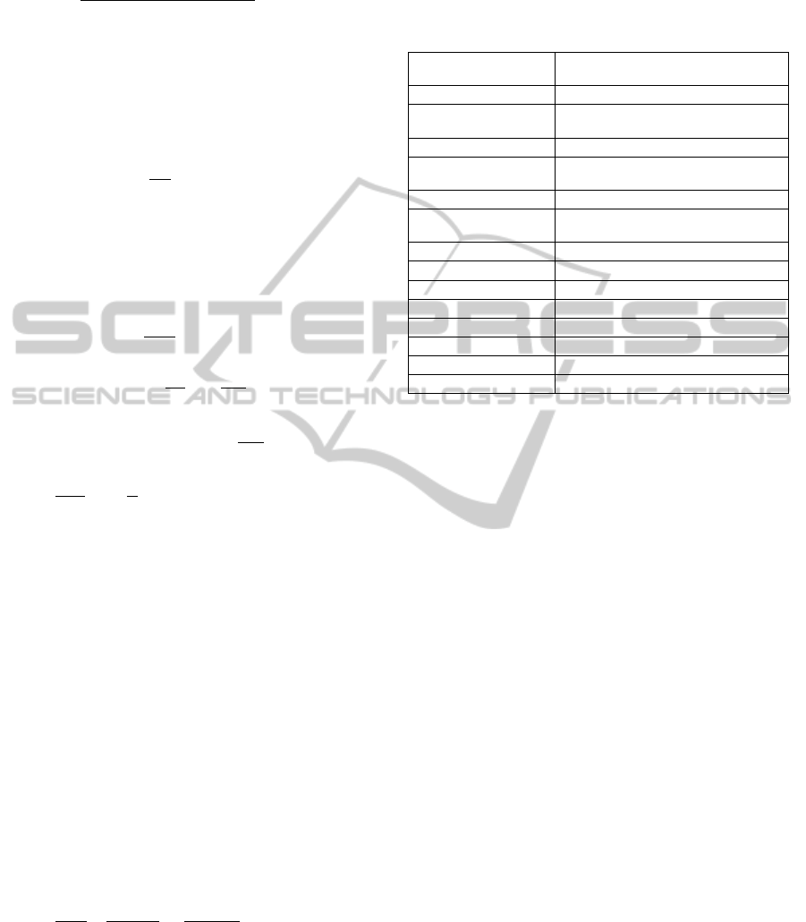
2.4 Computational Setup
This simulated object is a lab-scale fluidized bed
gasifier whose details can be found elsewhere (Lv,
2004). A schematic diagram of the reactor and the
simulation grid are shown in Fig. 1. The
experimental setup parameters and the operating
conditions appear in Table 2. At the outlet, gas phase
adopts out-flow boundary condition and no particle
exit. The reactor is initially filled with N
2
and the
silica sand is in the vessel with the volume fraction
grids of 0.48 (Wang, 2009). To prevent excessive
compression of particles, we set the solid close pack
volume fraction as 0.5. The particle normal-to-wall
momentum retention coefficient is 0.2 and the
tangent–to-wall retention coefficient is 0.99. The
time step of 2.0×10
-4
s is used.
Eulerian-Lagrangian Modeling of Forestry Residues Gasification in a Fluidized Bed
299
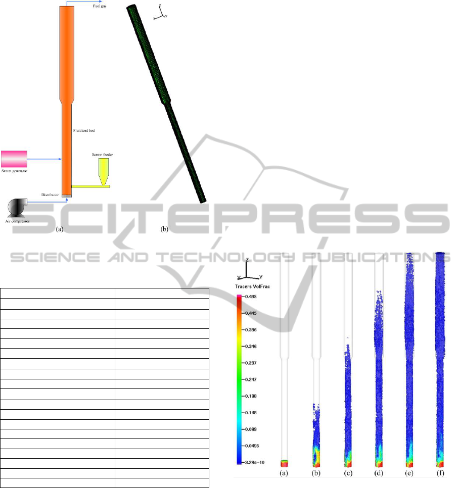
Figure 1: Schematic of the gasifier and simulation grid.
Table 2: Experimental setup parameters and operating
conditions.
Fluidized bed reactor
Temperature (℃)
750,800,850
Pressure (Pa)
101325
Bed diameter (mm)
40
Freeboard diameter (mm)
60
Height (mm)
1400
Air
Temperature (℃)
65
Flow rate (Nm
3
/h)
0.5
Steam
Temperature (℃)
154
Flow rate (kg/h)
1.2
Feed material: Pine sawdust
Particle diameter (mm)
0.3-0.45
Absolute density (kg/m3)
556
Char density (kg/m3)
1300
Flow rate (kg/h)
0.445
Bed material : Silica sand
Particle diameter (mm)
0.2-0.3
Weight (g)
30g
3 RESULTS AND DISCUSSION
3.1 Flow Patterns
In the fluidized bed, air was used as the fluidizing
agent and introduced into the reactor below the
distributor. The particles include three species: silica
sand, carbon and ash. The formation and
development of granular flow regimes are illustrated
with particle volume fraction in Fig. 2. As shown in
Fig. 2(a)-(f), the particles tend to rise with time
driven by gas-particle interactions. The particle
concentration decreases along the reactor height.
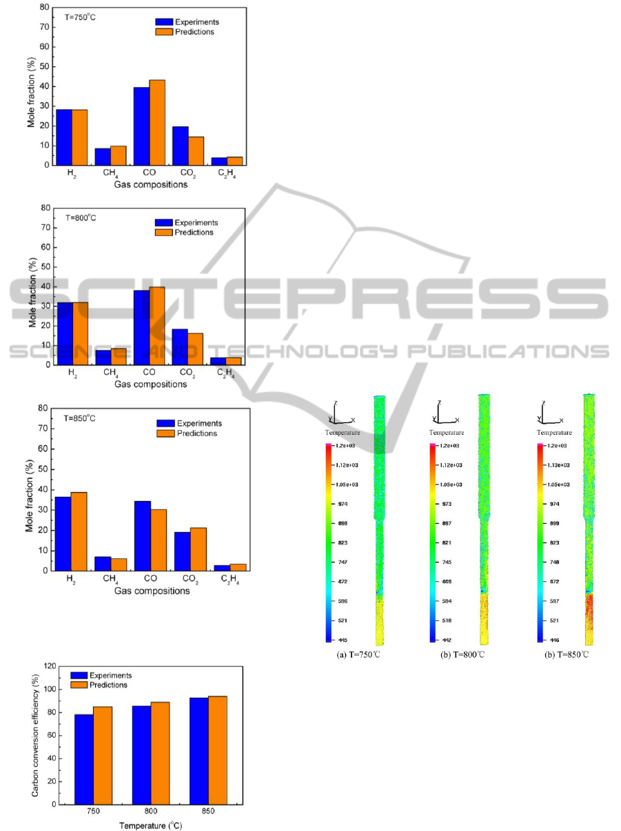
3.2 Comparisons with Experiments
The present developed model was applied to three
cases with different operating temperatures. Fig. 3
portrays the product gas composition of calculations
and experiment data. All species are dry-gas molar
contents.
Fig. 3(a)-(c) shows the predicted results compare
well with the experimental data. The minimum
relative error is less than 1%, and the maximum
relative error is about 20%. The average relative
error is less than 12%.Very little difference is found
between predicted and measured H
2
, CH
4
and C
2
H
4
contents. The H
2
concentrations increase with
increasing temperature and the contents of CH
4
show
an opposite trend. Higher temperature favors the
endothermic reaction of methane steam reforming.
Figure 2: Flow patterns transition with time: (a) t=0s, (b)
t=0.25s, (c) t=0.5s, (d) t=0.75s, (e) t=1.0s, (f) t =1.25s.
One or two calculation error of CO and CO
2
molar
contents are more than 15%. The reason for these
deviations is likely to be the simplified distribution
coefficient of reactions: C +
O
2
→ (2-
) CO
2
+
(2-2
) CO
and C + αH
2
O → (2-α) CO + (α-1) CO
2
+
αH
2
, the coefficients, α and
, change with
temperature which are set as constants in our model.
Part of the deviation comes from the neglect of tar
production.
SIMULTECH 2012 - 2nd International Conference on Simulation and Modeling Methodologies, Technologies and
Applications
300
(a)
(b)
(c)
Figure 3: Comparisons between species mole contents
predicted by model and experimental data.
Figure 4: Comparisons between carbon conversion
efficiency predicted by model and experimental data.
Fig. 4 compares the predicted carbon conversion
efficiency with the measured data. Higher
temperature improves the gasification process and
increases the carbon conversion. There is good
agreement between the simulation and experimental
results. The average relative difference is only about
5%. Biomass produces tar and other light
hydrocarbon (C
x
H
y
) in pyrolysis and gasification
process. The present model did not consider the tar
and light hydrocarbon, which is the main reason for
over-estimation of carbon conversion efficiency.
3.3 Distributions of Gas Compositions
Fig. 5 displays the distributions of particle and gas
temperatures in the reactor (a half slice at y=0). In
general, the temperature in the bed region is higher
than in the freeboard for the more contact of
gasifying agent and fuel. The steam injection affects
the temperature profile and lowers the temperature
above the injection level. The peak temperatures are
observed in the lower part of the bed, where the
highest intensities of combustion and gasification
reactions are located.
Figure 5: Distributions of particle and gas temperatures.
Fig. 6 illustrates the molar fraction distribution of
the five most important gas species in the reactor (a
half slice at y=0). It can be seen from the figure: the
positions of the sawdust feeder and steam injector
influence the gas profile. Near the particle inlet level,
the molar concentrations of CO are highest due to
the existence of a large number of carbon particle
and devolatilization. The CO
2
concentrations remain
almost constant along the whole height of the reactor
for the homogeneous combustion reaction and
Eulerian-Lagrangian Modeling of Forestry Residues Gasification in a Fluidized Bed
301
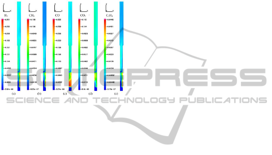
water-gas shift reaction. The overall trend of H
2
,
CH
4
and C
2
H
4
contents is consistent. As a result of
devolatilization, the peak concentrations of them are
presented close to the feeder. Nevertheless, H
2
molar
contents are higher than those of CH
4
and C
2
H
4
in
the freeboard region due to water-gas shift reaction
and methane steam reforming reaction.
Figure 6: Molar fraction distributions of gas compositions
(T=800℃).
4 CONCLUSIONS
A three-dimensional Eulerian-Lagrangian numerical
model was developed to study the forestry residues
gasification in a laboratory scale fluidized bed
gasifier. By the simulations at different operating
temperaures, gasifier’s behavior was effectively
predicted, including the complex particle flow
patterns, profile of temperature and distributions of
gas composition. The predicted product gas contents
and carbon conversion efficiency compared well
with experimental data. The present mathematical
model can be a tool to explore the complex gas-solid
flow and chemical reaction characteristics of
fluidized bed gasification.
ACKNOWLEDGEMENTS
Financial supports from the Major State Basic
Research Development Program of China (NO.
2011CB201505), China MOST for Inter-government
S&T Optional Cooperation between China and
Europe (2010DFA61960), NSFC (No. 51076029),
and UK EPSRC for Collaboration Project of China
and British (EP/G063176/1) were sincerely
acknowledged.
REFERENCES
Nemtsov, D. A., Zabaniotou, A., 2008. Mathematical
modelling and simulation approaches of agricultural
residues air gasification in a bubbling fluidized bed
reactor. Chemical Engineering Journal 143, 10–31.
Nikoo, M. B., Mahinpey, N., 2008. Simulation of biomass
gasification in fluidized bed reactor using ASPEN
PLUS. Biomass and Bioenergy 32, 1245–1254.
Gómez-Barea, A., Leckner, B., 2010. Modeling of biomass
gasification in fluidized bed. Progress in Energy and
Combustion Science 36, 444-509.
Snider, D. M., 2001. An incompressible three dimensional
multiphase particle-in-cell model for dense particle
flows. Journal of Computational Physics 170,
523-549.
Snider, D. M., 2007. Three fundamental granular flow
experiments and CPFD predictions. Powder
Technology 176, 36-46.
Snider, D. M., Clark, S. M., O’Rourke, P. J., 2011.
Eulerian-Lagrangian method for three-dimensional
thermal reacting flow with application to coal
gasifiers. Chemical Engineering Science 66,
1285-1295.
Thunman, H., Thunman, H., Niklasson, F., Johnsson, F.,
Leckner, B., 2001. Composition of Volatile Gases and
Thermochemical Properties of Wood for Modeling of
Fixed or Fluidized Beds. Energy Fuels 15, 1488-1497
de Souza-Santos, M. L.,. Modeling, Simulation, and
Equipment Operations. 2004. Marcel Dekker, Inc.
Lv, P. M., Xiong, Z. H., Chan, g J., Wu, C. Z., Chen, Y.,
Zhu, J. X., 2004. An experimental study on biomass
air–steam gasification in a fluidized bed. Bioresource
Technology 95, 95-101.
Wang, X. F., Jin, B. S., Zhong, W. Q., 2009.
Three-dimensional simulation of fluidized bed coal
gasification. Chemical Engineering and Processing 48,
695-705.
SIMULTECH 2012 - 2nd International Conference on Simulation and Modeling Methodologies, Technologies and
Applications
302
