Simulation and Multi-objective Optimization

of Vaccuum Ethanol Fermentation

Jules Thibault

, Rubens Maciel Filho

2,3

, Marina O. S. Dias

, Tassia L. Junqueira

2,3

, Otavio Cavalett

Charles D.F. Jesus

, Carlos E.V. Rossell

and Antonio Bonomi

Department of Chemical and Biological Engineering, University of Ottawa, Ottawa (Ontario), K1N 6N5, Canada

Faculdade de Engenharia Química, Departamento de Processos Químicos

Universidade Estadual de Campinas, R. Albert Einstein, nº 500,13081-970 - Campinas, SP - Brazil

Laboratório Nacional de Ciência e Tecnologia do Bioetanol - CTBE/CNPEM

Caixa Postal 617013083-970, Campinas, Brazil

Keywords: Ethanol Fermentation, in Situ Recovery, Vacuum Fermentation, Simulation, Optimization.

Abstract: With the overall objective of optimizing an integrated first and second generation bioethanol production

plant, a simple illustrative example is first used to examine the advantages and challenges of using a

combination of VBA and UniSim Design for multi-objective optimization. In this paper, the simulation and

optimization of a vacuum fermentation system using glucose and xylose as substrates is performed. The

simulation of the fermentation system and the optimization are performed in the VBA environment, while

UniSim Design is used to provide thermodynamic data necessary to perform calculations and used to

simulate the downstream portion of the fermentation vacuum system. The Pareto domain of the system was

circumscribed based on three decision variables (starting time of vacuum, rate of broth removal by vacuum

and condenser temperature) and four objective functions (minimum ethanol loss, maximum productivity,

minimum residual sugars and minimum compression energy). The procedure developed has allowed to

easily circumscribe the Pareto domain of this system and to observe clearly the compromises that are

required when all objective functions are optimized simultaneously. Some challenges to overcome are the

time required for exchanging information between VBA and UniSim Design and the risk of non-converging

for complex problems. For this procedure to be implemented effectively for the integrated ethanol plant,

some innovative measures need to be developed.

1 INTRODUCTION

As a mean of partially reducing the world

dependence on non-renewable petroleum as a fuel

source and overall carbon dioxide emissions,

research on biofuels has intensified significantly

during the last decade with the main focus placed on

bioethanol and biodiesel, and more recently on

biobutanol. In many industrialized countries, over

two thirds of the refined petroleum products sold is

used for transportation purposes (NRCan, 2009; U.S.

EIA, 2010). This includes gasoline, low-sulphur

diesel, and aviation fuel. There is therefore a need

for a transitional fuel that will allow for a smooth

changeover.

Bioethanol has great potential and has already

been blended with some mainstream fuel sources at

concentrations varying from 10% per volume up to

100%. Bioethanol has many advantages, including

reduced dependence on imported oil, new markets

for farmers and foresters, and a reduction of

greenhouse gas (GHG) emissions from vehicles.

Facing with the highly-publicized criticism of

diverting farmlands or crops away from the human

food chain supply (not the case for sugarcane), a

shift to second-generation biofuels and a greater use

of residual lignocellulosic biomass to produce

biofuels is well underway to partly reduce this

controversy.

The step before fermentation, to obtain

fermentable sugars, and the microorganisms used in

fermentation are the main differences between the

ethanol production processes from simple sugar,

starch or lignocellulosic material (Mussatto et al.,

2010). The production of bioethanol from

lignocellulosic biomass is significantly more

Thibault J., Maciel Filho R., O. S. Dias M., L. Junqueira T., Cavalett O., D. F. Jesus C., E. V. Rossell C. and Bonomi A..

Simulation and Multi-Objective Optimization of Vaccuum Ethanol Fermentation.

DOI: 10.5220/0004014400790086

In Proceedings of the 2nd International Conference on Simulation and Modeling Methodologies, Technologies and Applications (SIMULTECH-2012),

pages 79-86

ISBN: 978-989-8565-20-4

 2012 SCITEPRESS (Science and Technology Publications, Lda.)

complex and costly than the one from sugarcane and

corn (Krissek, 2008). Indeed the efficient conversion

of lignocellulosic biomass into fermentable sugar

remains a major challenge for commercial

application (Margeot et al., 2009). The impetus

nowadays is to have a more integrated plant with the

production of multiple products. In Brazil, current

bioethanol plants draw their revenues from sugar,

bioethanol and electricity. In newer plants, first and

second generation bioethanol production will

probably be integrated, taking advantage of sharing

part of the infrastructure and the feedstock

availability (bagasse and trash) for second

generation ethanol production (Dias et al., 2012).

The increased complexity of these plants requires

the system to be well optimized.

A research project has been initiated to optimize

the integrated ethanol plant. The complete integrated

plant has been simulated using Aspen Plus (Dias et

al., 2008). It is desired to use this simulated plant to

perform a multi-objective optimization of this plant

by integrating it into an optimization algorithm.

Various scenarios are currently envisaged to

determine how to best incorporate the simulated

plant. One scenario, which is the subject of this

paper, is to use Excel/VBA (Visual Basic for

Applications) as an optimization platform but also as

a communication platform for passing on arguments

to and retrieving information from Aspen HYSYS or

Honeywell UniSim Design.

Given the complexity of the simulated ethanol

integrated plant, it was decided to implement this

scenario progressively. As a first step, it was desired,

via a simple illustrative example, to examine how

the combination of Excel, VBA and UniSim Design

could be used for optimizing a vacuum ethanol

fermentation process with regards to the protocol of

communication, the ease of convergence and the

time required to converge to an optimized solution.

In this paper, a vacuum fermentation system is

simulated and optimized based on three decision

variables and four objective criteria. The paper is

organized as follows. First, the simulated

fermentation system will be described followed by

the description of the optimization procedure. Some

results will then be presented and discussed prior to

concluding.

2 FERMENTATION SYSTEM

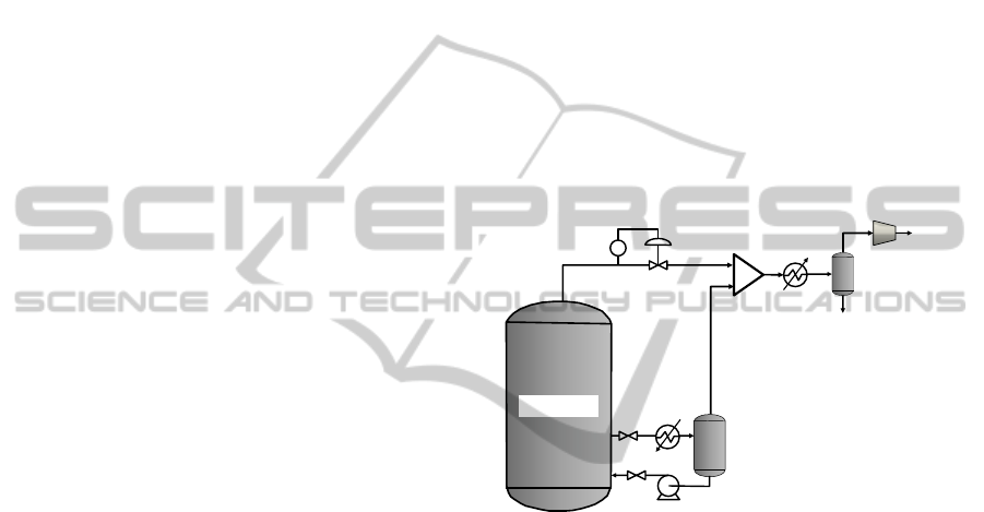
The simple illustrative process of Figure 1 consists

of a fermenter containing initially 500 m

inoculated fermentation medium. The initial

substrate concentrations of glucose and xylose in the

broth are 150 g/L and 75 g/L, respectively. A ratio

of 2:1 for glucose:xylose is typical of fermentable

sugars from lignocellulosic biomass. At this level of

substrate concentration, incomplete consumption

occurs because ethanol reaches a concentration level

that is completely inhibitory to the microorganism.

The in situ ethanol recovery from the fermentation

broth can partly mitigate product inhibition and

extend the fermentation, thereby allowing more

complete substrate utilization. Many methods have

been proposed to achieve this objective (Cardona

and Sanchez, 2007): liquid-liquid extraction (Jassal

et al., 2009), adsorption (Einicke et al., 1991), gas

stripping (Liu and Hsien-Wen, 1990), pervaporation

(Groot et al., 1992), and vacuum fermentation (Park

and Geng, 1992). In this investigation, a simplified

version of vacuum fermentation is simulated.

Figure 1: Simplified vacuum fermentation system.

The fermenter of Figure 1 operates at

atmospheric pressure but is equipped with an

external flash tank that, when in operation, is

maintained at a pressure low enough for the

fermentation broth to boil. When it is desired to

continuously remove a portion of ethanol from the

fermentation broth to reduce the inhibition, a small

stream of the fermentation broth is continuously

circulated through the external flash tank to be

partially evaporated. The heat exchanger preceding

the external flash tank serves to provide the latent

heat of vaporization of the evaporated fraction of the

stream and is used to control the rate of evaporation.

The exiting vapour is richer in ethanol such that the

in situ ethanol recovery is possible, resulting in a

decrease or a delay in fermentation inhibition caused

by ethanol accumulation. The exiting vapour passes

through a condenser to recover most of the

evaporated water and ethanol. In the present scheme,

in order to simplify the number of components, it

also was decided to send the CO

stream to the

Fermenter

Flash

Tank

Compressor

Condenser

Heater

SIMULTECH 2012 - 2nd International Conference on Simulation and Modeling Methodologies, Technologies and

Applications

condenser in lieu of having a separate absorption

column.

2.1 Fermentation Model

There are numerous models for predicting the

production and consumption of the main species

involved in fermentation. In this investigation, the

model of Leksawasdi et al. (2001) was used. This

model was developed for the batch fermentation of

mixtures of glucose and xylose by recombinant

Zymomonas mobilis strain ZM4(pZB5), containing

additional genes for xylose assimilation and

metabolism. The model represented very well

experimental biomass growth, utilization of the two

substrates and ethanol production over a large range

of substrate concentrations.

This model has been adopted in this investigation

to evaluate the in situ product recovery during

fermentation operating at 30

C. The microbial

growth on each sugar is modelled using Equation (1)

with index j being 1 for glucose and 2 for xylose,

respectively. This equation includes three terms

affecting the maximum growth rate: (1) Monod

kinetics for substrate limitation, (2) ethanol

inhibition with a threshold level and a maximum

inhibitory concentration, and (3) a typical substrate

inhibition term.

iX,j iX,j

X,j max,j

X,j j mX, j iX,j iX,j j

P - P K

r = 1 -

K + S P - P K + S



   

   

   

(1)

The total biomass growth based on these two

sugars is represented by Equation (2).

X,1 X,2

= r + (1 - )r X







(2)

The associated glucose and xylose consumption

rates are given in Equation (3).

iS,j iS,j

,max, j

SS,j j mS, j iS, j iS, j j

P - P K

dS S

= - 1- X

dt K +S P -P K +S



   

   

   

(3)

The rate of ethanol production can be related to

the rates of glucose and xylose consumption subject

to similar constraints and is given in Equation (4).

P,1 P,2

= r + (1 - )r X







(4)

with

iP,j iP,j

P,j ,max, j

SP,j j mP,j iP,j iP, j j

P - P K

r = 1 -

K + S P - P K + S

   

   

   

(5)

The model of Leksawasdi et al. (2001) did not

need to account for the production of carbon dioxide

during fermentation. However, in the present

investigation, it is necessary to know the amount of

carbon dioxide leaving the fermenter when vacuum

is used to reduce the concentration of ethanol in the

fermenter. We will assume that CO

is produced

according to stoichiometric equation for the

consumption of glucose and xylose. For each kg of

glucose or xylose consumed, 0.489 kg CO

produced. It is assumed that the same quantity of

is produced whether the substrate is used for

ethanol production or biomass. It is therefore

possible to write the following differential equation

to account for the rate of CO

produced.

dS dS

= - 0.489 +

dt dt dt







(6)

where dG/dt represents the mass rate of CO

production per unit volume of liquid broth.

The 31 parameters of the model can be found in

Leksawasdi et al. (2001). With these parameters and

the three sets of initial conditions given in the paper,

it was possible to reproduce exactly the curves

appearing in the publication.

2.2 Simulation Details

To perform the optimization of the process (covered

in the next section), the simulation of the complete

system must be performed numerous times with

different input design parameters. It is not possible

to perform the fermentation simulation within

UniSim Design such that the simulation of the

majority of the system and the optimization

algorithm were performed in the VBA environment

and UniSim Design was used as a supporting

platform for thermodynamic calculations and for

simulating the immediate downstream part of the

process. The simulation subroutine first obtains from

an EXCEL spreadsheet the initial conditions of the

fermenter content: X

(0.028 kg/m

), S

(150

kg/m

), S

(75 kg/m

), P

(0 kg/m

), fermentation

time (40 h) and the volume (500 m

). A schematic

diagram of the interaction between these computer

programs is presented in Figure 2.

Figure 2: Diagram of simulation communication protocol.

The fermentation is initiated in batch mode such

that the system of Equations (1)-(6) is integrated

numerically. An additional term in the mass

balances for the batch fermentation was added to

Excel UniSim

Object

Library

Object

Library

VBA

Simulation and Multi-Objective Optimization of Vaccuum Ethanol Fermentation

account for the entrainment of ethanol and water

from the fermenter due to carbon dioxide exiting the

fermenter. It is assumed that the carbon dioxide gas

stream leaves the fermenter saturated in ethanol and

water. When the external flash tank is put in

operation, an additional term to the mass balance of

each differential equation is added to account for the

evaporation rates of ethanol and water.

For each integration step of the mass balance

differential equations, the vapour partial pressure of

ethanol and water is calculated by passing to UniSim

Design the concentration of the fermentation broth

and by retrieving the equilibrium mass fraction in

the vapour phase (stream 1). With this information,

it is possible to perform a complete mass balance for

each species within the fermenter and to calculate

the mass flow rate and composition of streams 1 and

2 (Figure 1). The information of the combined

stream 3 and the desired exit temperature of stream 4

are then sent to UniSim to perform heat and mass

balances and to calculate the mass flow rates and

concentrations of streams 5, 6 and 7. VBA then

retrieves these flow rates and concentrations in

addition to the energy required for cooling stream 3

and the power required by the compressor. A

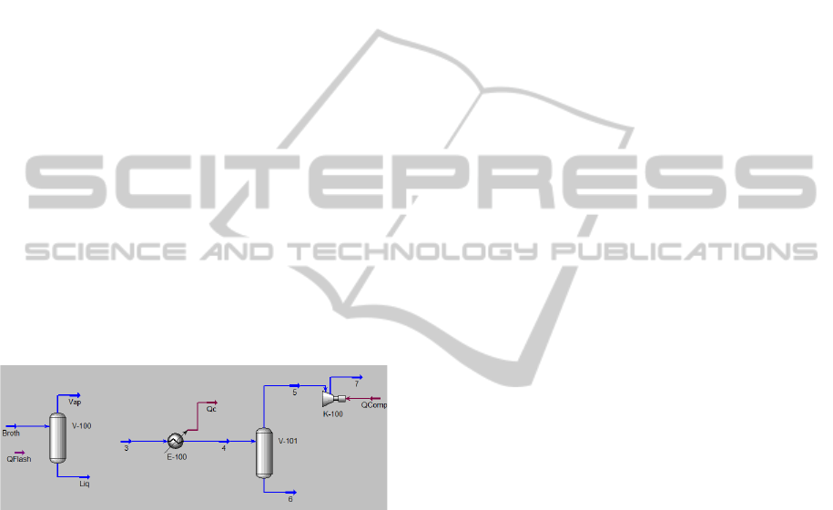
screenshot of the two simple systems used in

UniSim Design is shown in Figure 3.

Figure 3: UniSim Design screen capture showing the two

processes supporting VBA simulation.

3 OPTIMIZATION ALGORITHM

3.1 Multi-Objective Optimization

The first step to optimize a process is choosing a set

of process decision variables that can be

manipulated and that have an effect on a series of

objective functions. The choice of these decision

variables and objective functions need to be

performed by experts who have a profound

knowledge of the process. In the simple vacuum

fermentation illustrative example, three decision

variables were first considered (ranges of variation

in brackets): (1) the time at which the vacuum

system is placed in operation [0, 40 h], (2) the

evaporation rate in the external vacuum flash tank

[0, 6 m

/h], and (3) the exit temperature of the

condenser (stream 4) [-10, 10

C].

For this optimization study, four objective

functions were retained: (1) minimization of overall

ethanol lost (kg), i.e. the cumulative amount of

ethanol leaving stream 7, (2) maximization of

overall ethanol productivity (kg/m

h) based on

initial fermenter volume, (3) minimization of

residual sugars at the end of fermentation (kg), and

(4) minimization of the average consumption by the

compressor (MJ/h). This selection is of course not

unique and, ideally, the amortized total capital and

operating costs per kg of ethanol produced could

also need to be considered. However, to investigate

the benefits and constraints of using a combination

of EXCEL-VBA-UniSim Design, the current

example meets this requirement. As mentioned, this

simple example must be viewed as a preliminary

exploration for the optimization of the complete

integrated ethanol plant.

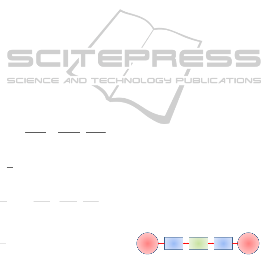
This problem, as summarized in Figure 4, is a

multi-objective optimization system. It is desired to

determine the values of the decision variables that

will maximize the second objective function while

minimizing the other three functions. It is possible to

combine the four objective functions into a single

profit function to be minimized. Even though single

objective optimization has been often used in the

literature, this method suffers from several

disadvantages such as the lack of information about

the trade-offs amongst various competing objectives,

the difficulty to assign the relative weighting to each

individual objective in a single profit function and

the convergence on a suboptimal point (local

maximum or minimum) instead of global optimum

in complex nonlinear problems (Deb, 2001; Haupt

and Haupt, 2004).

Even though it requires more computation time,

it is significantly more informative to solve the

problem as a multi-objective problem with the

distinct advantage to generate multiple Pareto-

optimal solutions that provide the decision maker or

expert a global perspective about trade-offs between

conflicting objectives. Other advantages include the

ability to optimize functions without requiring

information about function derivatives and therefore

application in non-convex, non-concave and

discontinuous problems (Deb, 2001; Haupt and

Haupt, 2004).

SIMULTECH 2012 - 2nd International Conference on Simulation and Modeling Methodologies, Technologies and

Applications

Figure 4: Schematic optimization block flow diagram of

the decision variables and objective functions.

3.2 Pareto Domain

The Pareto domain is the set of all feasible solutions

that are non-dominated by other solutions in that set.

A solution X

is said to dominate another solution X

if the values of all objectives for X

are not worse

than those of X

, and the value of at least one

objective for X

is better than the corresponding X

(Deb, 2001). Otherwise, both points are non-

dominated relative to each other.

Different algorithms exist in the literature to

circumscribe the Pareto domain from an initial

population of solutions. In this investigation, the

dual population evolutionary algorithm (DPEA) was

used. This algorithm incorporates the concepts of

domination to generate the Pareto domain. The

general approach is briefly described as follows

(Perrin et al., 1997; Thibault, 2008):

1. An initial set of decision variables is randomly

generated within their specified ranges. For each

of these points, the values of the objective

functions are then calculated as per Section 3.1.

2. The objective functions of all the points are

compared to the others (one solution versus

another at a time) to determine the number of

times a solution is dominated by another.

3. The non-dominated solutions of the population

and a portion of the least dominated solutions are

used to generate new solutions to replace

discarded solutions. To generate a new solution,

two kept solutions are chosen randomly and a

linear interpolation of their decision variables is

performed and the objective functions are

calculated.

4. The procedure is repeated until the desired

number of non-dominated individuals in the

population is obtained.

When the Pareto domain is circumscribed, it can

be used per se or the solutions can be ranked

according to some preferences expressed by an

expert. Two methods are particularly efficient to

capture preferences of experts: Net Flow Method

and Rough Set Method (Thibault, 2008). In this

investigation, only the Pareto domain will be

circumscribed and analyzed.

4 RESULTS AND DISCUSSION

4.1 Simulation Statistics

For each function call of the optimizing subroutine,

the set of mass balance equations for the

fermentation system was integrated over a period of

40 h with a time step of 0.1 h for a total 400

integration steps. Under ideal conditions, it takes

approximately 16 to 20 s of computation time to

simulate the 40 h fermentation on a Lenovo laptop

computer with an Intel 2.49GHz Dual Processor.

Sometimes it took much longer to complete a

simulation run. The difference in time required

undoubtedly depends on the ease to converge to a

solution within UniSim even though the flowsheet is

relatively simple. The majority of this time is spent

communicating with UniSim Design and performing

calculation within UniSim. Indeed, to perform a

complete function call without resorting to UniSim

took less than 1 s.

When the correct communication protocol has

been established between VBA and UniSim Design,

the simulation of a complete fermentation run was

possible and the optimization routine was able to

properly approximate the Pareto domain. To obtain a

population of 242 non-dominated solutions, it took

more than 1500 function calls. A higher number of

function calls are required when the number of

objective functions is higher. It requires significantly

more function calls than a traditional optimization

method but it is believed that the payback in having

the possibility to examine the trade-offs expressed

by the Pareto domain is all worth it.

The use of a metamodel is currently being

explored to converge more rapidly to the final Pareto

domain. In this method, a neural network model

representing the underlying relationship between the

decision variables and the objective functions would

be developed using the information of the initial

population. The metamodel would then be used in

the optimization method to determine the Pareto

domain. Finally, the Pareto domain obtained using

the metamodel would be validated and refined using

the more accurate original model. The development

of convergence promoter tools is important if one

wants to tackle the optimization of the complete

ethanol plant in the future. Other techniques are also

being evaluated.

4.2 Pareto Domain

A Pareto domain is specific to a set of decision

variables and objective functions. Changing some of

Vacuum

Fermentation

System

Vac

Out

Ethanol loss

Ethanol productivity

Residual sugars

Energy of compressor

Simulation and Multi-Objective Optimization of Vaccuum Ethanol Fermentation

the decision variables and/or objective functions will

lead to a different Pareto domain. All solutions

within the Pareto domain are non-dominated

solutions such that in the pairwise comparison of

any two solutions, each solution is better for at least

one objective function. All feasible solutions outside

the Pareto domain are dominated which means that

there exists at least one point within the Pareto

domain that is better for all four objective criteria.

The main advantage of the Pareto domain is the

possibility to clearly observe the compromises that

are being made when trying to optimize all four

objective functions at the same time. The resulting

Pareto domain is a four-dimensional surface

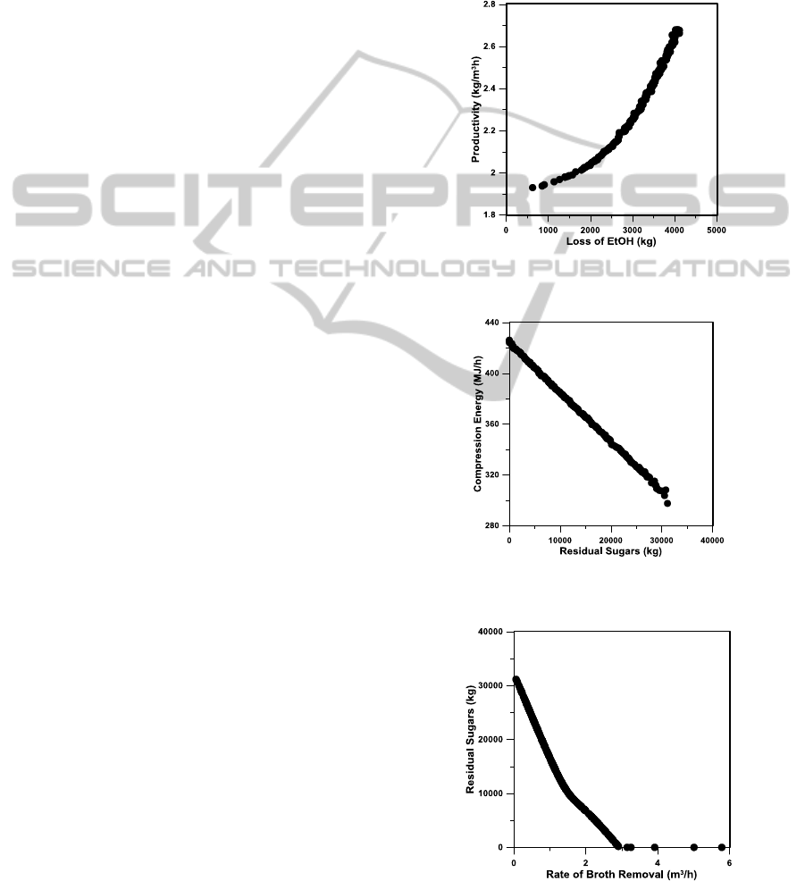
containing all potential optimal solutions. Figures 5

and 6 present the four objective functions of the

Pareto domain using two-dimensional projections.

Each of the 242 points on the graphs represents a

different fermentation simulated with a different set

of decision variables (start time for vacuum,

evaporation rate and condenser temperature).

Figure 5 illustrates very well the compromises

that the Pareto domain expresses where an increase

in the productivity is accompanied by a greater loss

of ethanol. Similar compromise is expressed in

Figure 6 where the minimization of residual sugars

leads to an increase in the power of compression.

Two main reasons explain this compromise: (1) the

utilization of a greater quantity of xylose and

glucose leads to a higher production of carbon

dioxide, and (2) a greater sugar consumption rate

requires a higher removal rate of ethanol from the

broth in order to reduce product inhibition as shown

in Figure 7. Figure 7 shows very clearly that to

completely use glucose and xylose by reducing

product inhibition, the minimum fermentation

removal rate in the flash tank must be nearly 3 m

when the flash tank vacuum system is put into

operation. Similarly (plots not shown), increasing

productivity is accompanied by a decrease in

residual sugars and increase in compression energy.

In this investigation, for simplicity and to reduce

the number of pieces of equipment, the carbon

dioxide stream was combined to the evaporated

broth stream. Using a traditional absorption column

to capture ethanol would reduce the power of

compression at the expense an additional column.

Information about the decision variables are

presented in Figures 8 and 9. The histogram of

Figure 8 reveals that for the majority of the solutions

within the Pareto domain, the vacuum flash tank was

put into operation in the vicinity of 20 h, in fact 21.1

± 5.8 h. This is where the level of ethanol

concentration starts to have a greater inhibiting

effect and some of it needs to be removed. It is

also more efficient to remove ethanol when the

concentration is higher. It would be possible to

refine the optimization by adding a stopping time for

the vacuum system as another decision or,

alternatively, adding the total fermentation time as a

decision variable. Either addition would have for

benefit to reduce the energy required for

compression.

Figure 5: Plot of ethanol productivity versus total ethanol

loss during fermentation.

Figure 6: Plot of the energy required for compression

versus the residual sugars at the end of fermentation.

Figure 7: Plot of residual sugars versus rate of broth

removal via vacuum boiling.

SIMULTECH 2012 - 2nd International Conference on Simulation and Modeling Methodologies, Technologies and

Applications

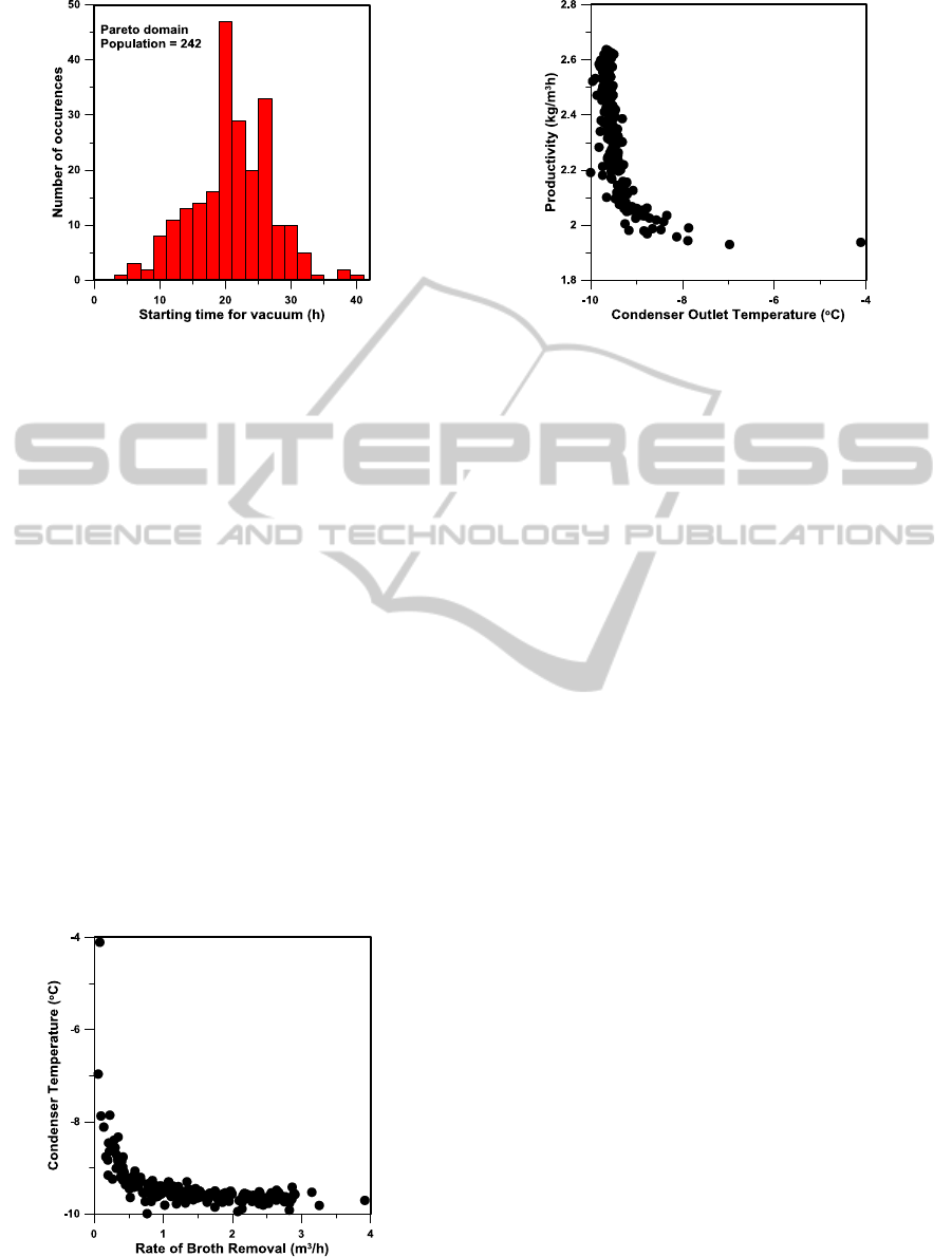
Figure 8: Histogram of the time at which the vacuum flash

tank is put into operation for Pareto-optimal solutions.

Figure 9 shows that as the rate of broth removal

via the vacuum flash tank is increased, the

temperature of the condenser needs to be lowered.

For most of the Pareto domain, the condenser

temperature hovers in the vicinity of its lower limit

of -10

C. Of course, a lower condensing temperature

will lead to lower ethanol loss but at greater

refrigerant expenses. A lower condensing

temperature leads to a higher productivity as shown

in Figure 10.

The current fermentation model was developed

for a fermenter operating at 30

C such that low

vacuum pressure due to thermodynamic limitation

had to be used to perform in situ ethanol recovery. If

the fermentation could occur at a higher

temperature, higher pressure could be used thereby

significantly reducing the cost. Microorganisms able

to tolerate higher fermentation temperature are

currently available but the productivity is yet too

low to compete with existing technology (Kumar et

al., 2010).

Figure 9: Plot the condenser outlet temperature versus the

rate of broth removal.

Figure 10: Plot of productivity versus condenser outlet

temperature.

5 CONCLUSIONS

The main goal of this paper was to examine, via the

simulation and optimization of a simple illustrative

example, the ease of combining Excel, VBA and

UniSim Design for optimizing industrial plants. This

investigation has shown that even for a simple

system, the time to access UniSim Design to pass

and retrieve information is relatively long. To

optimize a more complex plant, the time of

simulation will be a limiting factor with the

additional risk of not converging to a solution within

UniSim Design. It will be necessary to resort to

innovative and efficient methods to be able to

perform the optimization of a complex plant such as

the integrated first and second generation ethanol

production plant.

In this investigation, the bulk of the simulation

and optimization of the vacuum fermentation system

was performed within VBA with UniSim Design

performing thermodynamic and downstream

processing calculations. The Pareto domain was

circumscribed and allowed to observe very clearly

the compromises that need to be made when four

objective functions, mostly conflicting, were

optimized simultaneously.

ACKNOWLEDGEMENTS

The financial contribution of the Canadian National

Science and Engineering Research Council

(NSERC) is acknowledged.

Simulation and Multi-Objective Optimization of Vaccuum Ethanol Fermentation

REFERENCES

Cardona, C. A., Sanchez, O. J. 2007. Fuel ethanol

production: Process design trends and integration

opportunities. Bioresource Technology, 98,

2415-2457.

Deb, K. 2001. Multi-objective optimization using

evolutionary algorithms. New York: Wiley.

Dias, M. O. S., Maciel Filho, R., Maciel, M. R. W.,

Rossell, C.E.V., Bioethanol production from

sugarcane and sugarcane bagasse investigation of plant

performance and energy consumption. 18

International Congress of Chemical and Process

Engineering - CHISA, 2008.

Dias, M. O. S., Junqueira, T. L., Cavalett, O., Cunha, M.

P., Jesus, C. D. F., Rossell, C. E. V., Maciel Filho, R.,

Bonomi, A. 2012. Integrated versus stand-alone

second generation ethanol production from sugarcane

bagasse and trash. Bioresource Technology, 103, 152-

161.

Einicke, W.D., Gläser, B., Schöoullner, R. 1991. In-Situ

recovery of ethanol from fermentation broth by

hydrophobic adsorbents. Acta Biotechnologica, 11(4),

353-358.

Groot, W. J., Kraayenbrink, M. R., Waldram, R. H., Lans

R. G. J. M., Luyben K. Ch. A. M. 1992. Ethanol

production in an integrated process of fermentation

and ethanol recovery by pervaporation. 8, 99-111.

Haupt, R. L. and Haupt, S. E. 2004. Practical Genetic

Algorithms, 2

Ed., John Wiley & Sons.

Kumar, S, Singh, S.P., Mishra, I.M., Adhikari, D.K. 2010.

Feasibility of ethanol production with enhanced sugar

concentration in bagasse hydrolysate at high

temperature using Kluyveromyces sp. IIPE453.

Biofuels, 1(5), 697-704.

Jassal, D.S., Zhang, Z., Hill, G.A. 2009. In-situ extraction

and purification of ethanol using commercial oleic

acid. Can. J. Chem. Eng., 72(5), 822-827.

Krissek, G. 2008. Future Opportunities and Challenges for

Ethanol Production and Technology. http://www.

farmfoundation.org/news/articlefiles/378-Krissek%

202-5-08.pdf.

Leksawasdi, N., Joachimsthal, E.L., Rogers, P.L. 2001.

Mathematical modelling of ethanol production from

glucose/xylose mixtures by recombinant Zymomonas

mobilis. Biotechnology Letters 23: 1087–1093.

Liu, H.S., Hsien-Wen, H. 1990. Analysis of gas stripping

during ethanol fermentation - I. In a continuous stirred

tank reactor. Chemical Engineering Science. 45(5),

1289-1299.

Mussatto, S.I., Dragone, G., Guimarães P.M.R., Silva,

J.P.A., Carneiro, L.M., Roberto, I.C., Vicente, A.,

Domingues, L., Teixeira, J.A. 2010. Technological

trends, global market, and challenges of bio-ethanol

production

Nguyen, V.D., Kosuge, H., Auresenia, J., Tan, R.,

Brondial, Y. 2009. Effect of vacuum pressure on

ethanol fermentation. Journal of Applied Sciences,

9(17), 3020-3026.

NRCan (March 24, 2009). Energy Sources. Consulted

August 5, 2011. Natural Resources Canada:

http://www.nrcan.gc.ca/eneene/sources/pripri/aboapr-

eng.php.

NRCan (January 4, 2011). Personal: Transportation.

Consulted August 8, 2011.Natural Resources Canada:

http://oee.nrcan.gc.ca/publications/infosource/pub/vehi

clefuels/ethanol/M92_257_2003.cfm.

Margeot, A., Hahn-Hagerdal, B., Edlund, M., Slade, R.,

Monot, F.. 2009. New improvements for

lignocellulosic ethanol, Curr. Opinions. Biotechnol.,

20, 372–380.

Park, C. H., Geng, Q. 1992. Simultaneous Fermentation

and Separation in the Ethanol and Abe Fermentation.

Separation and Purification Reviews, 21(2) 127-174.

Perrin, E., Mandrille, A., Oumoun, M., Fonteix, C., Marc,

I. (1997). Optimization globale par stratégie

d'évolution: Technique utilisant la Génétique des

individus diploides. RAIRO- Recherche Operationelle

31, 161-201.

Thibault, J. (2008). Net Flow and Rough Sets: Two

Methods For Ranking the Pareto Domain. In G.

Rangaiah (Ed.), Chapter 7 - Multi-Objective

Optimization: Techniques and Applications in

Chemical Engineering. World Scientific Publishing.

U.S. EIA (August 2010). Annual Energy Review

2009.ConsultedAugust 5, 2011, www.eia.gov/aer.

SIMULTECH 2012 - 2nd International Conference on Simulation and Modeling Methodologies, Technologies and

Applications