
Automatic Subspace Clustering with Density Function
Jiwu Zhao and Stefan Conrad
Institute of Computer Science, Databases and Information Systems, Heinrich-Heine University,
Universitaetsstr.1, 40225 Duesseldorf, Germany
Keywords:
Subspace Clustering, Density Function, High Dimension.
Abstract:
Clustering techniques in data mining aim to find interesting patterns in data sets. However, traditional cluster-
ing methods are not suitable for large, high-dimensional data. Subspace clustering is an extension of traditional
clustering that enables finding clusters in subspaces within a data set, which means subspace clustering is more
suitable for detecting clusters in high-dimensional data sets. However, most subspace clustering methods usu-
ally require many complicated parameter settings, which are always troublesome to determine, and therefore
there are many limitations for applying these subspace clustering methods. In this article, we develop a novel
subspace clustering method with a new density function, which computes and represents the density distri-
bution directly in high-dimensional data sets, and furthermore the new method requires as few parameters as
possible.
1 INTRODUCTION
Usually, we need to investigate unknown or hidden
information from raw data. Clustering techniques
help us to discover interesting patterns in the data
sets. Clustering methods divide the observations into
groups (clusters), so that observations in the same
cluster are similar, whereas those from different clus-
ters are dissimilar. Clustering is important for data
analysis in many fields, including market basket anal-
ysis, bio science, and fraud detection. Clustering also
provides foundations for other data mining tasks, such
as classification and association.
Unlike traditional clustering methods that seek
clusters only in the whole space, subspace cluster-
ing enables clustering in particular projections (sub-
spaces) within a data set, which means that the clus-
ters could be found in subspaces rather than only in
the whole space.
Although most subspace clustering algorithms can
find clusters in subspaces of a data set, the effectiv-
ity is a problem of these algorithms. For instance,
it is commonly known that the majority of the algo-
rithms usually demand many parameter settings for
high-dimensional data sets. However, the values of
these parameters are hard to determine. In addition,
because of their sensitivities to the parameter values,
these algorithms often generate very different cluster-
ing results of the data sets.
In this paper, we introduce a novel subspace clus-
tering algorithm, which is a density-based clustering
method. It calculates the distribution of data sets with
its denstiy function, and clusters are explored in order
of cluster sizes. The method can be applied for differ-
ently scaled data. Moreover, the algorithm uses one
parameter, which simplifies the application process.
The remainder of this paper is organized as fol-
lows: In section 2, we present related work in the
area of subspace clustering, and some similar ideas
from other algorithms. Section 3 describes our new
subspace clustering method. Section 4 presents ex-
perimental studies for verifying the proposed method.
Finally, section 5 contains some conclusions together
with some ideas for further works.
2 RELATED WORK
In recent years, there is an increasing amount of
literature on subspace clustering. Surveys such as
those conducted by Parsons (Parsons et al., 2004) and
Kriegel (Kriegel et al., 2009) have divided subspace
clustering algorithms into two groups: top-down and
bottom-up. Top-down methods (e.g. PROCLUS (Ag-
garwal et al., 1999), FINDIT (Woo et al., 2004), σ-
Clusters (Yang et al., 2002)) use multiple iterations
for improving the clustering results. By contrast,
bottom-up methods (e.g. CLIQUE (Agrawal et al.,
63
Zhao J. and Conrad S..
Automatic Subspace Clustering with Density Function.
DOI: 10.5220/0004031400630069
In Proceedings of the International Conference on Data Technologies and Applications (DATA-2012), pages 63-69
ISBN: 978-989-8565-18-1
Copyright
c
2012 SCITEPRESS (Science and Technology Publications, Lda.)

1998), ENCLUS (Cheng et al., 1999), MAFIA (Goil
et al., 1999)) firstly find clusters in low subspaces, and
then expand the search by adding more dimensions.
However, all the previously mentioned subspace
clustering methods suffer from some serious limita-
tions related to determination of proper values for
their parameters. For instance, parameters of top-
down methods (e.g. numbers of clusters and sub-
spaces) and the bottom-up method’s parameters (e.g.
density, grid interval, size of clusters) influence the
iterations and clustering results, however the parame-
ters cannot be determined easily. In order to make the
clustering task more practical, it is necessary to find
an easier way to determine the parameters.
DENCLUE (Hinneburg et al., 1998) is a density-
based clustering algorithm that uses Gaussian ker-
nel function as its abstract density function and hill
climbing method to find cluster centers. DENCLUE
2.0 (Hinneburg and Gabriel, 2007) is an improvement
on DENCLUE, which does not have to estimate the
number or the position of clusters, because cluster-
ing is based on the density of each point. However,
it is still necessary to estimate the parameters in the
algorithms, such as mean and variance in DENCLUE
or the iteration threshold and the percentage of the
largest posteriors in DENCLUE 2.0. Besides, they
are not designed for subspace clustering.
DBSCAN (Density-Based Spatial Clustering of
Applications with Noise) (Ester et al., 1996) is a
density-based clustering algorithm because it finds
clusters by estimating density distribution of corre-
sponding nodes. The definition of a cluster in DB-
SCAN is based on the notion of density-reachability.
A cluster of DBSCAN satisfies two properties: All
objects within the cluster are density-connected; If an
object is density-connected to any object in a cluster,
it belongs to the cluster as well. DBSCAN requires
two parameters: the minimum distance for neigh-
borhood (ε) and the minimum number of objects for
forming a cluster (minPts). SUBCLU (Kr
¨
oger et al.,
2004) is a subspace clustering algorithm based on
DBSCAN. SUBCLU uses a bottom-up, greedy strat-
egy to find clusters in subspaces. In the first step
of SUBCLU, all one-dimensional subspaces are clus-
tered, then all clusters in a (k + 1)-dimensional sub-
space will be built from k-dimensional ones. Simi-
lar to DBSCAN, SUBCLU takes also two parameters
ε and minPts, however, one issue of SUBCLU is to
choose the two parameters properly for data with dif-
ferent value ranges.
In previous work we introduced a subspace
clustering method SUGRA (Zhao, 2010) (subspace
clustering method by using gravitation’s function).
SUGRA applies a density function that is similar to
gravitation function for the purpose of representing
the density distribution in each single dimension and
locating the clusters in high-dimensional subspaces.
A cluster object in high density area has a high value
of density, meanwhile a non cluster object has al-
ways a low value. We could find the cluster objects
according to this property. SUGRA works well in
many situations, however for the high-dimensional
subspace it is a little complex, since the combination
of the objects in high-dimensional subspace from one-
dimensional objects is not the best solution.
For the purpose of establishing a method for a
convenient and practical application in subspace clus-
tering, we introduce here a novel subspace cluster-
ing algorithm, which is named Automatic Subspace
Clustering with Distance-Density function (ASCDD).
ASCDD’s density function is an improvement of the
gravitation function in SUGRA. Moreover, the idea is
also inspired from DBSCAN, in ASCDD the cluster
objects are considered as density-connected, however
the criterion for density-connectivity is different from
DBSCAN. ASCDD needs just one parameter in order
to make the clustering process as simple and accurate
as possible.
3 CLUSTERING PROCESS
Generally, a data set could be considered as a pair
(
e
A,
e
O), where
e
A = {a
1
,a
2
,···} is a set of all at-
tributes (dimensions) and
e
O = {o
1
,o
2
,···} is a set of
all objects. o
{a
j
}
i
denotes the value of an object o
i
on
dimension a
j
.
A subspace cluster S is also a data set and can be
defined as follows: S = (A, O), where the subspace
A ⊆
e
A and O ⊆
e
O, and S must satisfy a particular con-
dition C , which is defined differently in each subspace
clustering method, however, a general principle of C
is that objects in the same cluster are similar, mean-
while the ones from different clusters are dissimilar.
S
A
indicates subspace clusters that refer to A.
Compared with other algorithms, we pay more
attention to the high-dimensional subspaces and try
to apply a density function directly to the objects in
any high-dimensional subspace. The density function
should have the properties: There are significant dif-
ferences in density values between dense objects and
not dense objects; Moreover, the scale of density val-
ues should not depend on the types or scales of the
objects, e.g. no matter clustering salary or length the
density values should have the same range. It is also
desirable that the density values of objects for any
subspaces should remain in the same range.
DATA2012-InternationalConferenceonDataTechnologiesandApplications
64
SUGRA has a density function suitable for an one-
dimensional space. We developed the density func-
tion of ASCDD from SUGRA, so that the density
function of ASCDD can be applied for calculating the
density values directly to objects in any subspace.
One important definition in ASCDD is distance-
density. The definition of distance-density is based
on the Euclidian distance with the property of mea-
suring density of two objects relative to all objects.
In order to unite the data with different scales in
each subspace, the first step is normalizing the ob-
jects in each dimension, and the normalization of an
object o
i
in one dimension a is defined as ¯o
{a}
i
=
o
{a}
i
−min(o
{a}
)
max(o
{a}
)−min(o
{a}
)
. Obviously, every object has a value
¯o
{a}
i
∈ [0,1] through the normalization. For conve-
nience, o
{a}
i
(value of object o
i
on dimension a) used
in the following is normalized. The distance-density
of objects o
i
and o
j
with regards to subspace A is de-
fined as follows:
d
A
o
i
,o
j
=
1
r
A
o
i
,o
j
2
· |
e
O| +1
2
(1)
where r
A
o
i
,o
j
is the normalized Euclidian dis-
tance, which is calculated as follows: r
A
o
i
,o
j
=
r
∑
∀a∈A
(o
{a}
i
− o
{a}
j
)
2
. It is evident that r
A
o
i
,o
j
∈
[0,
p
|A| ]. |
e
O| is the number of objects and has
a value 1. So that the distance-density d
A
o
i
,o
j
∈
h
1
(|A|·|
e
O|)
2
,1
i
. d
A
o
i
,o
j
varies inversely with r
A
o
i
,o
j
, which
means the smaller r
A
o
i
,o
j
, the closer d
A
o
i
,o
j
to 1.
Compared with SUGRA’s density function, if
r
A
o
i
,o
j
= 0, which means if the distance between two
objects is zero, the distance-density d
A
o
i
,o
j
= 1, how-
ever SUGRA has to treat this case specially. Another
advantage is that the density function can be applied
not just in one-dimensional subspace, but also in any
subspace A, because r
A
o
i
,o
j
is the normalized Euclidian
distance in the subspace. From the experiments, we
can see that the density function of ASCDD is more
efficient for high-dimensional subspaces.
The density of an object o
i
relating to all objects
in subspace A is defined as follows:
D
A
o
i
=
∑
∀o
j
d
A
o
i
,o
j
=
∑
∀o
j
1
r
A
o
i
,o
j
2
· |
e
O| +1
2
(2)
This density can be considered as a relative density,
which can be imagined as the ratio of a local distance
to sum of distance from all objects. The density dis-
tribution is determined from all the objects, however
the density of a single object is particularly influenced
by its local environment. For example, the density of
an object will get higher by putting more objects near
it, but the densities of objects at a far distance will
change very few.
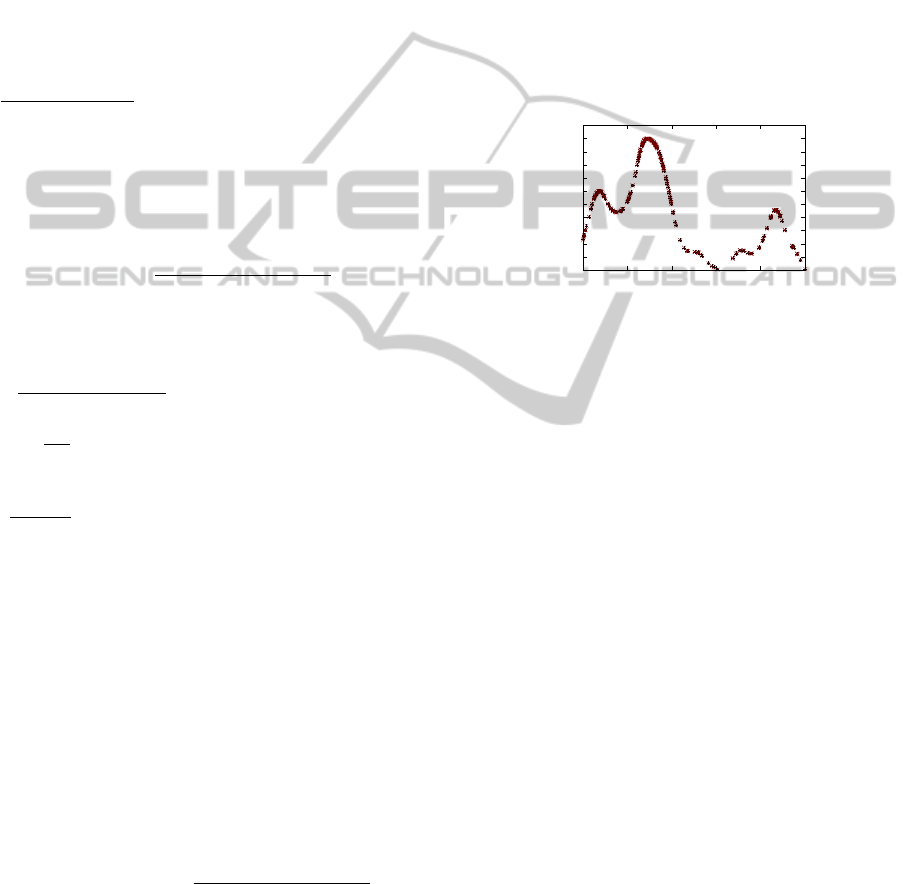
The density of an object reveals the amount of sur-
rounding objects and reflects a distribution of the ob-
jects, moreover the density at the center of a cluster
can indicate the size of the cluster. Figure 1 illustrates
an example of positions and densities of objects in an
one-dimensional space. It can be seen that, the larger
a cluster is, the higher density the central object has,
namely the peaks indicate centers of clusters, mean-
while the non cluster objects are always in the valley.
5
10
15
20
25
30
35
40
45
50
55
60
0 0.2 0.4 0.6 0.8 1
Density
Position of the objects
Figure 1: An example of density function.
The density function is a smooth function, how-
ever the differences of densities between cluster ob-
jects and non cluster objects are adequate for distin-
guishing clusters. Hence the density function is not
only just for observing the clusters clearly but also
the foundation for clustering process.
After calculating the distance-density, the next
question is how to find clusters from the density val-
ues. It is noteworthy that the objects at center of
a cluster are close to each other. Meanwhile, the
distance-density at the edge between cluster objects
and the objects outside the cluster are much sparser.
We consider that all objects in a cluster are neighbors,
so our idea for clustering is to search the neighbors of
center objects.
An important procedure in ASCDD is to check
whether two objects are neighbors. It should be
pointed out that the distance-densities for all objects
in different subspaces have a unified range. Consid-
ering this property we apply the distance-density for
neighborhood decision. The set of neighbors of an
object o
A
i
(Neighbor(o
A
i
)) is defined as follows:
d
A
o
i
,o
j
> DDT =⇒ o
A
j
∈ Neighbor(o
A
i
) (3)
Where DDT (distance-density threshold) is a thresh-
old for choosing the proper neighbors with distance-
density higher than DDT . As mentioned before,
d
A
o
i
,o
j
≤ 1, consequently the parameter DDT has also
to be determined with the value DDT < 1. It is appar-
AutomaticSubspaceClusteringwithDensityFunction
65
ent that the greater DDT is chosen, the fewer neigh-
bors are selected. It is important to choose an appro-
priate DDT for clustering. DDT is the only parameter
applied in the whole algorithm for the purpose of fa-
cilitation of choosing parameters.
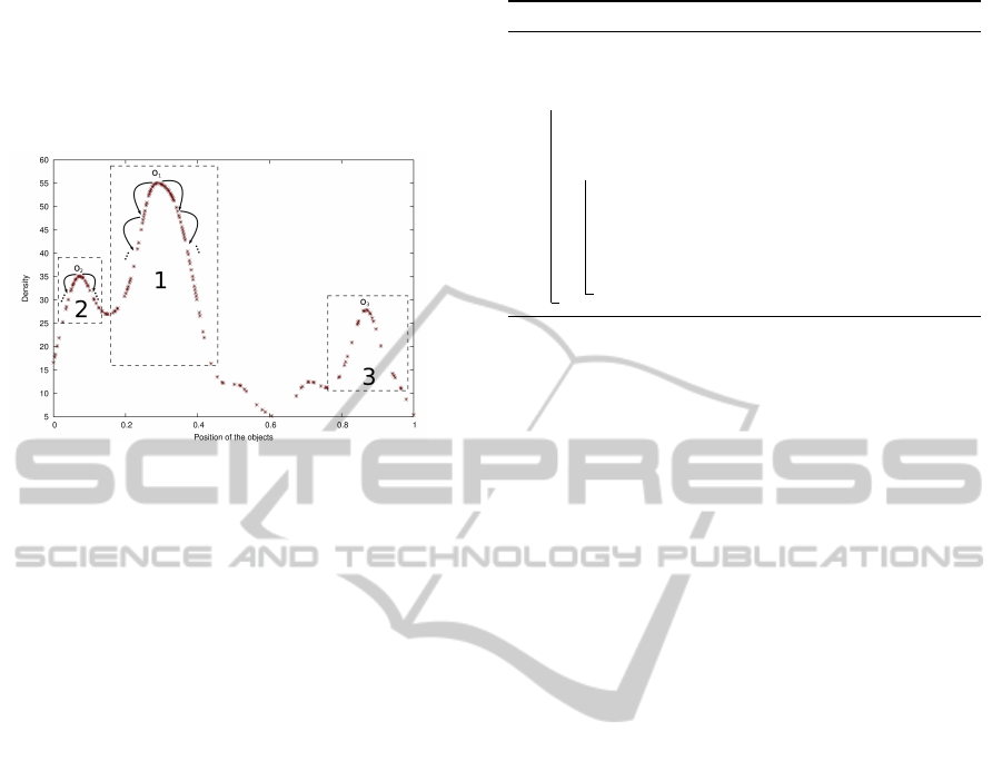
Figure 2: An example of clustering process of ASCDD.
In ASCDD, exploring a cluster begins with
searching neighbors of its center object, e.g. o
A
i
,
all objects in Neighbor(o
A
i
) belong to this clus-
ter, then ∀o
A
j
∈ Neighbor(o
A
i
)/{o
A
i
}, we search
Neighbor(o
A
j
) and insert the new objects into the
same cluster. Iteratively, each new object is searched
for its neighbors in the cluster until no further new
neighbor is found. Then, all objects in Neighbor(o
A
i
)
generate a cluster with the center object o
A
i
.
ASCDD firstly finds an object with the maximum
density, then searches the cluster related to the object,
after that it finds the next object with the maximum
density value from the rest of objects namely the next
center of a cluster. The same process repeats until all
clusters are found with descending sizes.
Figure 2 shows an example of a one-dimensional
clustering process. In this example, the clustering
process starts from object o
1
, which has maximum
density, and searches all neighbors of o
1
and sets them
as cluster 1, then cluster 1 will be extended by search-
ing new neighbors of current objects in this cluster.
The extension of cluster 1 will stop until no further
new neighbor is found. After we get cluster 1, all the
objects of cluster 1 are not considered for other clus-
ters, then the next object with the highest density is
o
2
, which is the center of cluster 2. The clustering
process of cluster 2 is the same as for cluster 1. Then
cluster 3 is on its turn, and so on. Finally, the clusters
are explored in turn according to their sizes.
3.1 Algorithm
The clustering process of ASCDD with respect to A
is divided into four steps.
Algorithm 1: ASCDD.
Input: (
e
A,
e
O)
Output: All S
1 foreach possible A ⊆
e
A do
2 O
current
=
e
O
3 ∀i, calculate D
A
o
i
4 while O
current
6=
/
0 do
5 o
A
s
has max(D
A
o
i
), ∀o
A
i
∈ O
current
6 O = Neighbor(o
A
s
)
7 Iteration: ∀o
A
i
∈ O, Neighbor(o
A
i
) ⊆ O
8 S = (A,O )
9 O
current
= O
current
− O
I. ∀i, Calculate D
A
o
i
.
II. Take the starting object o
A
s
that has the maxi-
mum density of current set of objects O
current
.
III. Find all neighbors from o
A
s
, and set them as a
cluster S, then expand S by finding new neigh-
bors of objects in S until no new neighbor is
found.
IV. Remove objects in S from O
current
, repeat step II
until no new cluster is found.
Obviously the neighbors distribute around their
center objects, however a cluster could have any form
by expanding its members’ neighbors, which could
reach all area and connect the cluster objects together.
Compared with k-means algorithm (MacQueen,
1967) or its variations, ASCDD does not have to con-
jecture the quantity of clusters, because the object
with the highest density as a starting object indicates
the center of each cluster already. The centers of clus-
ters emerge along with clustering gradually, which
means no matter how many clusters there are, all clus-
ters are searched one by one according to their densi-
ties, which is independent of the input order.
The density function of ASCDD can be consid-
ered as a distribution function, which describes the
distribution smoothly. The density function smoothes
out small local peaks, which are usually not necessary
to be considered in the clustering process. However,
the main characters of clusters are shown through the
density evidently, namely the cluster center has higher
density than objects at edge, and therefore the posi-
tion and size of the clusters can be indicated easily.
Another important feature is that the algorithm can be
applied directly in arbitrary subspaces, which is es-
pecially simple and convenient for direct clustering
particular subspaces.
Although ASCDD can be applied in any subspace,
directly applying ASCDD in all possible subspaces
would cause a calculation in O(2
|
e
A|
). There are many
feature selection methods for choosing relevant sub-
DATA2012-InternationalConferenceonDataTechnologiesandApplications
66
spaces from a data set. Our current approach seek
firstly all one-dimensional spaces with clusters. All
these one-dimensional spaces together are then taken
as candidate subspaces, and other subspaces are elim-
inated. From the candidate subspaces, we search
all possible subspace clusters from high to low sub-
spaces. This approach needs still to be optimized in
our future works.
4 EMPIRICAL EXPERIMENTS
4.1 Synthetic Data
In order to clearly illustrate the clustering result by
a graph, the experiment is carried out on a two-
dimensional space. For the purpose of testing accu-
racy, the clusters are set beforehand.
The synthetic data in the experiment is a simu-
lation about “galaxy stars”. The data set has 8372
objects, the clustering process took 72 seconds, the
experimental data and clustering result are shown in
Figure 3, where it can be seen that the black objects
are outliers and the cluster objects are marked with
different colors. The clustering result shows great ac-
curacy, moreover it is clear that any form including
concave form can be detected correctly.
0
0.2
0.4
0.6
0.8
1
0
0.2
0.4
0.6
0.8
1
Figure 3: Clustering result with “Galaxy”.
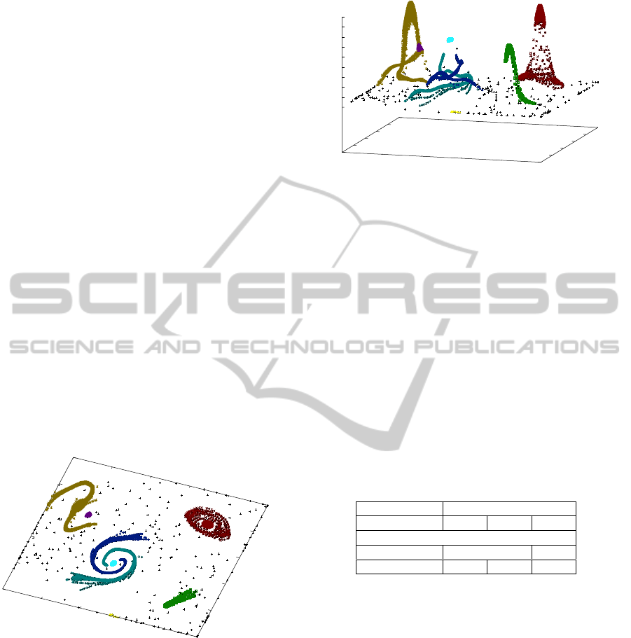
Figure 4 illustrates the densities of objects in three
dimensional space. Axis z shows that all objects’ den-
sities are greater than 0. The curve of the density
function represents the distribution of the objects very
clearly. The densities at the middle of the clusters are
much higher than the densities on the edge. The out-
liers have densities very close to 0.
4.2 Real Data
The data “wine” has been obtained from the UC
Irvine Machine Learning Repository (Frank and
0
0.2
0.4
0.6
0.8
1
0
0.2
0.4
0.6
0.8
1
0
100
200
300
400
500
600
700
800
900
Figure 4: Clustering result demonstrates in 3D.
Asuncion, 2010). This data set corresponds to the
analysis of wines derived from three different culti-
vars. There are 13 dimensions with three clusters
(with 59, 71 and 48 objects). Each dimension mea-
sures a constituent of the three types of wines.
The subspace clusters are detected in many sub-
spaces. We illustrate two examples of the clustering
result and their accuracies in Table 1. For instance, by
applying ASCDD directly on 13 dimensional space,
we found two subspace clusters S
1
, S
2
, where S
1
cor-
responds to the original clusters S
a
and S
b
together,
and S
2
corresponds to S
c
. The clustering uses 0.05
second. In the second example, we found three clus-
ters S
3
, S
4
and S
5
on the subspace {3,7,12,13}, the
accuracy of each cluster is shown in the table. This
clustering process takes 0.04 second.
Table 1: Accuracy of ASCDD on “wine”.
Number of objects in cluster
Wine S
a
(59) S
b
(71) S
c
(48)
ASCDD results:
A = {1, ··· ,13} S
1
(108) S
2
(46)
A = {3, 7,12,13} S
3
(51) S
4
(48) S
5
(47)
From the clustering results obtained, it shows that
the clustering results of ASCDD are quite close to the
original clusters. The clustering implemented directly
on high-dimensional subspace, and furthermore the
running time for high-dimensional subspace is still
very low.
4.3 Comparison with SUBCLU
Compared with SUBCLU (Kr
¨
oger et al., 2004), AS-
CDD needs to adjust one parameter DDT , where
SUBCLU has to set two parameters: minimum
distance ε and minimum number minPts. SUB-
CLU is a bottom-up algorithm, which starts cluster-
ing from one-dimensional space, and then searches
high-dimensional subspace cluster based on lower-
dimensional subspace clusters. Like SUBCLU, AS-
AutomaticSubspaceClusteringwithDensityFunction
67

CDD can also work with the bottom-up principle. We
apply the same synthetic data sets on ASCDD and
SUBCLU in order to compare the performances of
the two algorithms.
The experiment data sets has ten dimensions and
1000 objects. In the first test we set five simple clus-
ters in different subspaces. The ten dimensions have
the same value ranges. By choosing the proper param-
eters both algorithms yield almost the same results.
Both methods find the five clusters. The running
time is also similar for two methods. It is notewor-
thy that as the dimensionality of subspace increases,
the parameter settings are changing. The setting of
ε and minPts for SUBCLU is quite difficult by high-
dimensional subspace, whereas in ASCDD, DDT is
relatively simple to choose, because DDT should al-
ways be selected between 0 and 1.
In the second experiment, we change the ten-
dimensional data with various value ranges. In this
case, SUBCLU can not continue to work in the sub-
space higher than four dimension, because in high
dimensional all objects appear to be sparse, and the
strategy of choosing the minimum distance ε for
neighborhood becomes less efficient. However AS-
CDD works still excellent in this situation, and has no
trouble to discover the five subspace clusters exactly.
5 CONCLUSIONS
In this paper, we proposed a novel subspace clustering
method (ASCDD) based on former work (SUGRA)
for high-dimensional data set. Departing from the tra-
ditional clustering method, ASCDD can be applied
much easier with just one simple parameter and pro-
vides useful distribution information, and is suitable
for different types of data. The result of ASCDD is ac-
curate, and presents clusters according to their sizes,
which does not depend on the input order. Compare
with its predecessor SUGRA, ASCDD can investi-
gate clusters directly in high-dimensional subspace,
and moreover, the density function is smoother than
SUGRA’s.
From the results obtained so far, ASCDD works
really good in most situations. However, the clus-
tering result and quality depends on choosing the pa-
rameter DDT . Thus one extension of the approach is
researching a proper range of choosing DDT , which
will bring more convenience for the clustering pro-
cess. Another plan for our future work is to opti-
mize the subspace selection and to reduce the calcu-
lation time as the number of objects and dimensions
increases.
REFERENCES
Aggarwal, C. C., Wolf, J. L., Yu, P. S., Procopiuc, C., and
Park, J. S. (1999). Fast algorithms for projected clus-
tering. In Proceedings of the 1999 ACM SIGMOD in-
ternational conference on Management of data, SIG-
MOD ’99, pages 61–72. ACM.
Agrawal, R., Gehrke, J., Gunopulos, D., and Raghavan, P.
(1998). Automatic subspace clustering of high dimen-
sional data for data mining applications. In Proceed-
ings of the 1998 ACM SIGMOD international confer-
ence on Management of data, SIGMOD ’98, pages
94–105. ACM.
Cheng, C.-H., Fu, A. W., and Zhang, Y. (1999). Entropy-
based subspace clustering for mining numerical data.
In Proceedings of the fifth ACM SIGKDD interna-
tional conference on Knowledge discovery and data
mining, KDD ’99, pages 84–93. ACM.
Ester, M., Kriegel, H.-P., Sander, J., and Xu, X. (1996).
A density-based algorithm for discovering clusters in
large spatial databases with noise. In KDD, pages
226–231.
Frank, A. and Asuncion, A. (2010). UCI machine learning
repository. [http://archive.ics.uci.edu/ml]. University
of California, Irvine, School of Information and Com-
puter Sciences.
Goil, S., Nagesh, H., and Choudhary, A. (1999). Mafia:
Efficient and scalable subspace clustering for very
large data sets. Technical Report CPDC-TR-9906-
010, Northwestern University.
Hinneburg, A. and Gabriel, H.-H. (2007). Denclue 2.0: fast
clustering based on kernel density estimation. In Pro-
ceedings of the 7th international conference on Intel-
ligent data analysis, IDA’07, pages 70–80. Springer-
Verlag.
Hinneburg, A., Hinneburg, E., and Keim, D. A. (1998).
An efficient approach to clustering in large multime-
dia databases with noise. In Proc. 4rd Int. Conf. on
Knowledge Discovery and Data Mining, pages 58–65.
AAAI Press.
Kriegel, H.-P., Kr
¨
oger, P., and Zimek, A. (2009). Clustering
high-dimensional data: A survey on subspace cluster-
ing, pattern-based clustering, and correlation cluster-
ing. ACM Transactions on Knowledge Discovery from
Data, 3:1:1–1:58.
Kr
¨
oger, P., Kriegel, H.-P., and Kailing, K. (2004). Density-
connected subspace clustering for high-dimensional
data. In Proc. SIAM Int. Conf. on Data Mining
(SDM’04), pages 246–257.
MacQueen, J. B. (1967). Some methods for classification
and analysis of multivariate observations. In Proc. of
the fifth Berkeley Symposium on Mathematical Statis-
tics and Probability, volume 1, pages 281–297. Uni-
versity of California Press.
Parsons, L., Haque, E., and Liu, H. (2004). Subspace clus-
tering for high dimensional data: A review. SIGKDD
Explor. Newsl., 6:90–105.
Woo, K.-G., Lee, J.-H., Kim, M.-H., and Lee, Y.-J. (2004).
Findit: a fast and intelligent subspace clustering algo-
DATA2012-InternationalConferenceonDataTechnologiesandApplications
68

rithm using dimension voting. Information and Soft-
ware Technology, 46(4):255–271.
Yang, J., Wang, W., Wang, H., and Yu, P. (2002). δ-clusters:
Capturing subspace correlation in a large data set. In
Data Engineering, 2002. Proceedings. 18th Interna-
tional Conference on, pages 517 –528.
Zhao, J. (2010). Automatic parameter determination in sub-
space clustering with gravitation function. In Proceed-
ings of the Fourteenth International Database En-
gineering and Applications Symposium, IDEAS ’10,
pages 130–135. ACM.
AutomaticSubspaceClusteringwithDensityFunction
69
