View-based SLAM using Omnidirectional Images

D. Valiente, A. Gil, L. Fern

andez and O. Reinoso

System Engineering Department, Miguel Hern

andez University, 03202 Elche (Alicante), Spain

Keywords:

Visual SLAM, Omnidirectional Images.

Abstract:

In this paper we focus on the problem of Simultaneous Localization and Mapping (SLAM) using visual infor-

mation obtained from the environment. In particular, we propose the use of a single omnidirectional camera

to carry out this task. Many approaches to visual SLAM concentrate on the estimation of the position of a

set of 3D points, commonly denoted as visual landmarks which are extracted from images acquired at the

environment. Thus the complexity of the map computation grows as the number of visual landmarks in the

map increases. In this paper we propose a different representation of the environment that presents a series

of advantages compared to the before mentioned approaches, such as a simpliﬁed computation of the map

and a more compact representation of the environment. Concretely, the map is represented by a set of views

captured from particular places in the environment. Each view is composed by its position and orientation

in the map and a set of 2D interest points represented in the image reference frame. Thus, in each view the

relative orientation of a set of visual landmarks is stored. During the map building stage, the robot captures an

image and ﬁnds corresponding points between the current view and the views stored in the map. Assuming

that a set of corresponding points is found, the transformation between both views can be computed, thus

allowing us to build the map and estimate the pose of the robot. In the suggested framework, the problem

of ﬁnding correspondences between views is troublesome. Consequently, with the aim of performing a more

reliable approach, we propose a new method to ﬁnd correspondences between two omnidirectional images

when the relative error between them is modeled by a gaussian distribution which correlates the current error

on the map. In order to validate the ideas presented here, we have carried out a series of experiment in a

real environment using real data. Experiment results are presented to demonstrate the validity of the proposed

solution.

1 INTRODUCTION

The problem of SLAM is of paramount importance in

the ﬁeld of mobile robots, since a model of the en-

vironment is often required for navigation purposes.

The map building process is complex, since the robot

needs to build a map incrementally, while, simulta-

neously, computing its location inside the map. The

computation of a coherent map is problematic, since

the sensor data is corrupted with noise that affects the

simultaneous estimation of the map and the path fol-

lowed by the robot.

To the present days, approaches to SLAM can

be classiﬁed according to the kind of sensor data

used to estimate the map, the representation of the

map and the basic algorithm used for its computa-

tion. For example, due to their precision and robust-

ness, laser range sensors have been used extensively

to build maps (Stachniss et al., 2004; Montemerlo

et al., 2002). In this sense, two map representations

have been typically used: 2D occupancy grid maps

with raw laser (Stachniss et al., 2004), and the extrac-

tion of features from the laser measurements (Monte-

merlo et al., 2002) that are used to build 2D landmark-

based maps.

A subarea in the SLAM community proposes the

utilization of visual information to build the map.

These approaches use cameras as the main sensor and,

in consequence are usually denoted as visual SLAM.

Cameras possess a series of features that make them

attractive for its application to the SLAM problem.

However, vision sensors are generally less precise

than laser sensors and the research focuses on the

methods to extract usable information for the SLAM

process.

In the latter group, we can ﬁnd a great variety

of camera arrangements. For example, stereo-based

approaches in which two calibrated cameras extract

3D relative measurements to a set of visual land-

marks, being each landmark accompanied by a visual

Valiente D., Gil A., Fernández L. and Reinoso O..

View-based SLAM using Omnidirectional Images.

DOI: 10.5220/0004031800480057

In Proceedings of the 9th International Conference on Informatics in Control, Automation and Robotics (ICINCO-2012), pages 48-57

ISBN: 978-989-8565-22-8

 2012 SCITEPRESS (Science and Technology Publications, Lda.)

descriptor computed from its visual appearance (Gil

et al., 2010b). In this approach a Rao-Blackwellized

particle ﬁlter is used to estimate the map and path fol-

lowed by the robots. Other approaches propose the

use of a single camera to estimate a map of 3D vi-

sual landmarks and the 6 DOF pose of the camera

(Davison and Murray, 2002) with an EKF-SLAM al-

gorithm. Each visual landmark is detected with the

Harris corner detector (Harris and Stephens, 1988)

and described with a grey level patch. Since the dis-

tance to the visual landmarks cannot be measured di-

rectly with a single camera, the initialization of the

3D coordinates of a landmark poses a problem. This

fact inspired the inverse depth parametrization ex-

posed in (Civera et al., 2008). A variation of the In-

formation Filter is used in (Joly and Rives, 2010) to

estimate a visual map using a single omnidirectional

camera and an inverse depth parametrization of the

landmarks. Also, in (Jae-Hean and Myung Jin, 2003)

two omnidirectional cameras are combined to obtain

a wide ﬁeld of view stereo vision sensor. In (Scara-

muzza, 2011), the computation of the essential ma-

trix between two views allows to extract the relative

motion between two camera poses, which leads to a

visual odometry. According to (Andrew J. Davison

et al., 2004), the performance of the single-camera

SLAM is improved when using a wide ﬁeld of view

lens, which suggests the use of an omni-directional

camera in visual SLAM, since, in this case, the hori-

zontal ﬁeld of view is maximum.

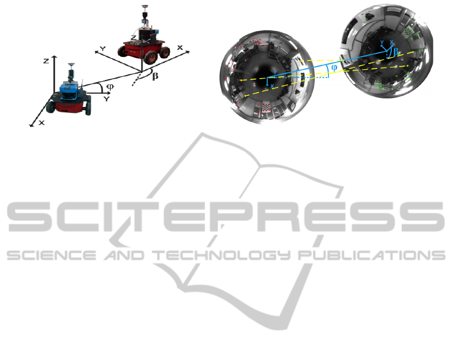
The approach presented in this paper assumes that

the mobile robot is equipped with a single omni-

directional camera. As shown in Figure 1(a), the opti-

cal axis of the camera points upwards, thus a rotation

of the robot moving on a plane is equivalent to a shift

along the columns of the panoramic image captured.

In this paper a different representation of the en-

vironment is proposed. To date, most of the work in

visual SLAM dealt with the estimation of the position

of a set of visual landmarks expressed in a global ref-

erence frame (Davison and Murray, 2002; Gil et al.,

2010b; Andrew J. Davison et al., 2004; Civera et al.,

2008). In this work, we concentrate on a different rep-

resentation of the environment: the map is formed by

the position and orientation of a set of views in the

environment. Each view is composed by an omnidi-

rectional image captured at a particular position, its

orientation in the environment and a set of interest

points extracted from it. Each interest point is accom-

panied by a visual descriptor that encodes the visual

appearance of the point. With this information stored

in the map, we show how the robot is able to build

the map and localize inside it. When the robot moves

in the neighbourhood of any view stored in the map

and captures an image with the camera, a set of in-

terest points will be matched between the current im-

age and the view. Next, a set of correspondences can

be found between the images. This information al-

lows us to compute the relative movement between

the images. In particular, the rotation between images

can be univocally computed, as well as the transla-

tion (up to a scale factor). To obtain these measure-

ments between images we rely on a modiﬁcation of

the Seven Point Algorithm (Scaramuzza et al., 2009;

Scaramuzza, 2011). This idea is represented in Fig-

ure 1(b), where we show two omnidirectional images

and some correspondences indicated. The transfor-

mation between both reference systems is also shown.

The computation of the transformation relies on the

existence of a set of corresponding points, thus, when

the robot moves away from the position of the stored

view, the appearance of the scene will vary and it may

be difﬁcult to ﬁnd any corresponding points. In this

case, a new view will be created at the current position

of the robot. The new initialized view allows for the

localization of the robot around its neighbourhood. It

is worth noting that a visual landmark corresponds to

a physical point, such as a corner on a wall. How-

ever, a view represents the visual information that is

obtained from a particular pose in the environment.

In this sense, a view is an image captured from a pose

in the environment that is associated with a set of 2D

points extracted from it. In the experiments we rely on

the SURF features (Bay et al., 2006) for the detection

and description of the points.

We consider that the map representation intro-

duced here presents some advantages compared to

previous visual SLAM approaches. The most impor-

tant is the compactness of the representation of the

environment. For example, in (Civera et al., 2008)

an Extended Kalman Filter (EKF) is used to estimate

the position of the visual landmarks, as well as the

position and orientation of the camera. With this rep-

resentation each visual landmarks is represented by

6 variables, thus the state vector in the EKF grows

rapidly as the number of visual landmarks increases.

This fact poses a challenge for most existing SLAM

approaches. In opposition with these, in the algo-

rithm presented here, only the pose of a reduced set

of views is estimated. Thus, each view encapsulates

information of a particular area in the environment, in

the form of several interest points detected in the im-

age. Typically, as will be shown in the experiments,

a single view may retain a sufﬁcient number of inter-

est points so that the localization in its neighbourhood

can be performed.

Storing only a set of views of the environment has,

however, some drawbacks. We have to face the prob-

View-basedSLAMusingOmnidirectionalImages

(a) (b)

Figure 1: Figure 1(a) shows the sensor setup used during the experiments. Figure 1(b) presents two real omnidirectional

images, with some correspondences indicated and the observation variables φ and β.

lem of determining a set of correspondences between

two views. Determining a metric transformation be-

tween two omnidirectional images is not trivial in the

presence of false data associations. However, in Sec-

tion 3 we present an algorithm that can be used to

process images at a fast rate for online SLAM. In this

case, the computation of the transformation between

two images depends only on the number of matches,

that can be easily adjusted to provide both speed and

precise results. Moreover we suggest a gaussian prop-

agation of the current error of the map in order to

come up with a reliable scheme of matching, so that

false correspondences are avoided.

We present a series of experiments and their re-

sults obtained trough the acquisition of real omnidi-

rectional images that demonstrate the validity of the

approach. The set of experiments have been carried

out by varying several parameters of the SLAM ﬁlter

when using real images captured in an ofﬁce-like en-

vironment. The paper is organized as follows: Sec-

tion 2 describes the SLAM process using the pro-

posed framework. Next, the algorithm used to esti-

mate the transformation between two omnidirectional

images is described in Section 3. Following, Section 4

presents the experimental results. Finally, Section 5

establishes a discussion to analyze the results.

2 SLAM

This section describes in detail the representation of

the environment as well as the map building process.

As mentioned before, the visual SLAM problem is

set out as the estimation of the position and orienta-

tion of a set of views. Thus, the map is formed by a

set of omnidirectional images obtained from different

poses in the environment. In opposition with other so-

lutions, the views do not correspond to any physical

landmarks or element in the environment (e.g. a cor-

ner, or the trunk of a tree). In our case, a landmark

(renamed view) will be constituted by an omnidirec-

tional image captured at the pose x

= (x

,θ

) and

a set of interest points extracted from that image.

In our opinion, this map representation can be

estimated using different kind of SLAM algorithms,

including online methods such as, EKF (Davison

and Murray, 2002), Rao-Blackwellized particle ﬁl-

ters (Montemerlo et al., 2002) or ofﬂine algo-

rithms, such as, for example, Stochastic Gradient De-

scent (Grisetti et al., 2007). In this paper we present

the application of the EKF to the proposed map rep-

resentation and explain how to obtain correct results

using real data.

In addition we consider that the map representa-

tion and the measurement model can be also applied

using standard cameras. The reason for using omni-

directional images is their ability to acquire a global

view of the environment in a single image, due to their

large ﬁeld of view, resulting in a reduced number of

variables to represent the map.

2.1 View-based Map

The pose of the mobile robot a time t will be denoted

as x

= (x

,θ

)

. Each view i ∈ [1,...,N] is con-

stituted by its pose x

= (x

,θ

)

, its uncertainty

and a set of M interest points p

expressed in im-

age coordinates. Each point is associated with a visual

descriptor d

, j = 1,...,M.

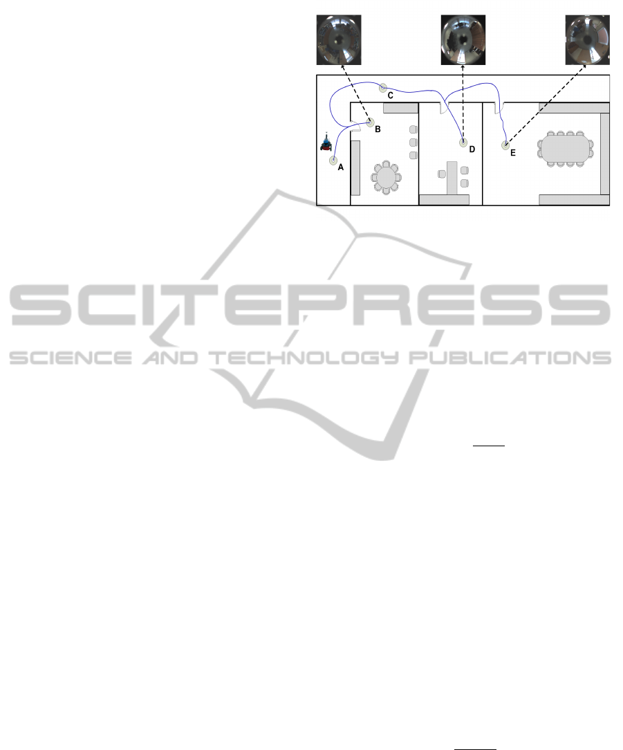
Figure 2 describes this map representation, where

the position of several views is indicated. For ex-

ample, the view A is stored at the pose x

,θ

)

in the map and has a set of M points

detected. The view A and C allow for the localization

of the robot in the corridor. The view B represents

the ﬁrst room, whereas the view D and E represent

the second and third room respectively, and make the

robot capable to localize in the environment.

ICINCO2012-9thInternationalConferenceonInformaticsinControl,AutomationandRobotics

Thus, the augmented state vector is deﬁned as:

¯x =



··· x



(1)

where x

= (x

,θ

)

is the pose of the moving ve-

hicle and x

= (x

,θ

) is the pose of the N-view

that exist in the map.

2.2 Map Building Process

This subsection introduces an example of map build-

ing in an indoor environment, represented in Figure 2.

We consider that the robot explores the environment

while capturing images with its omnidirectional cam-

era. The exploration starts at the origin denoted as A,

placed at the corridor. At this time, the robot captures

an omnidirectional image I

, that is stored as a view

with pose x

. We assume that, when the robot moves

inside the corridor, several point correspondences can

be found between I

and the current omnidirectional

image. Given this set of correspondences, the robot

can be localized with respect to the view I

. Next,

the robot continues with the exploration. When it en-

ters the ﬁrst room, the appearance of the images vary

signiﬁcantly, thus, no matches are found between the

current image and image I

. In this case, the robot

will initiate a new view named I

at the current robot

position that will be used for localization inside the

room. Finally, the robot keeps moving through the

corridor and goes into different rooms and creates

new views respectively at these points. The number

of images initiated in the map depends directly on the

kind of environment. In the experiments carried out

with real data we show that typically, a reduced num-

ber of views can be used while obtaining precise re-

sults in the computation of the map.

In addition, SLAM algorithms can be classiﬁed as

online SLAM when they estimate the map and the

pose x

at time t. Other algorithms solve the full

SLAM problem and estimate the map and the path

of the robot until time t, x

1:t

= [x

,...,x

]. The

EKF is generally classiﬁed in the ﬁrst group, since, at

each time t the ﬁlter gives an estimation of the cur-

rent pose x

. However, in our case, the position of

the view i coincides with the pose of the robot at any

of the views. In consequence the EKF ﬁlter allows

to compute the pose of the robot at time t and, in ad-

dition, a subset of the path followed by the vehicle

formed by the poses x

2.3 Observation Model

Following, the observation model is described. We

consider that we have obtained two different omni-

directional images captured at two different poses in

Figure 2: Main idea for map building. The robot starts the

exploration from A by storing a view I

. While the robot

moves and no matches are found between the current image

and I

, a new view is created at the current position of the

robot, for instance in B. The process continues until the

whole environment is represented

the environment. One of the images is stored in the

map and the other is the current image captured by the

robot at the pose x

. We assume that given two images

we are able to extract a set of signiﬁcant points in both

images and obtain a set of correspondences. Next, as

will be described in Section 3, we are able to obtain

the observation z





arctan(

−y

−x

) − θ

− θ

(2)

where the angle φ is the bearing at which the view

N is observed and β is the relative orientation be-

tween the images. The view N is represented by

= (x

,θ

), whereas the pose of the robot

is described as x

= (x

,θ

). Both measurements

(φ,β) are represented in Figure 1(a).

2.4 Initializing New Views in the Map

We propose a method to add new views in the map

when the appearance of the current view differs sig-

niﬁcantly from any other view existing in the map.

A new omnidirectional image is stored in the map

when the number of matches found in the neighbour-

ing views is low. Concretely, we use the following

ratio:

R =

+ n

(3)

that computes the similarity between views A and B,

being m the total number of matches between A and B

and n

the number of detected points in images

A and B respectively. The robot includes a new view

in the map if the ratio R drops below a pre-deﬁned

threshold. To initialize a new view, the pose of the

view is obtained from the current estimation of the

View-basedSLAMusingOmnidirectionalImages

robot pose and its uncertainty equals the uncertainty

in the pose of the robot.

3 COMPUTING A

TRANSFORMATION BETWEEN

OMNI-DIRECTIONAL IMAGES

In this section we present the procedure to retrieve the

relative angles β and φ between two omni-directional

images, as represented in Figure 1(b). As shown be-

fore, these angles compose the observation described

in (2). Computing the observation involves different

problems: ﬁrst, the detection of feature points in

both images and next, ﬁnding a set of point corre-

spondences between images that will be used to re-

cover a certain camera rotation and translation. Tradi-

tional schemes, such as (Kawanishi et al., 2008; Nis-

ter, 2003; Stewenius et al., 2006) apply epipolar con-

strains between both images and solve the problem in

the general 6 DOF case, whereas in our case, accord-

ing to the speciﬁc motion of the robot on a plane, we

reduce the problem to the estimation of 3DOF.

3.1 Detection of Interest Points

SURF features (Bay et al., 2006) are used to ﬁnd in-

terest points in the images and to describe their visual

appearance. In (Gil et al., 2010a), SURF features out-

perform other detectors and descriptors in terms of ro-

bustness of the detected points and invariance of the

descriptor. SURF features have been previously used

in the context of localization (Murillo et al., 2007) us-

ing omnidirectional images. We transform the om-

nidirectional images into a panoramic view in order

to increase the number of valid matches between im-

ages due to the lower appearance variation obtained

with this view.

3.2 Matching of Interest Points

In order to obtain a set of reliable correspondences be-

tween two views, several restrictions have to be con-

sidered. Some authors (Scaramuzza, 2011) rely on the

epipolar geometry to restrict the search of correspon-

dences. The same point detected in two images can

be expressed as p = [x, y, z]

in the ﬁrst camera refer-

ence system and p

= [x

]

in the second camera

reference system. Then, the epipolar condition estab-

lishes the relationship between two 3D points p and

seen from different views.

E p = 0 (4)

where the matrix E is denoted as the essential matrix

which can be computed from a set of corresponding

points in two images.

E =





0 0 sin(φ)

0 0 −cos(φ)

sin(β − φ) cos(β − φ) 0





(5)

being φ and β the relatives angles that deﬁne a pla-

nar motion between two different views, as shown in

Figure 1 and (2).

The epipolar restriction (4) has been previously

used to compute a visual odometry from two consec-

utive views (Scaramuzza, 2011), together with some

techniques such as RANSAC and Histogram voting to

reject false correspondences. In this sense, the com-

putation of the whole set of detected points is needed

in order to ﬁnd those which satisfy the restriction.

Moreover, in the context of visual odometry, consec-

utive images are close enough to disregard high er-

rors in the pose from where images were taken, so

that the epipolar restriction can be normally applied.

However, focusing on a SLAM framework, there ex-

ists uncertainties in the pose of the robot as well as

in the pose of the views that compose the map. For

this reason, we consider that is necessary to propa-

gate this errors to accomplish a reliable data asso-

ciation. We suggest using the predicted state vector

extracted from the Kalman ﬁlter, from which we are

able to obtain a predicted observation measurement

ˆz

by means of (2). In order to reduce the search of

valid corresponding points between images, the map

uncertainties have also to be taken into account, so

we propagate them to (4) by introducing a dynamic

threshold, δ. In a idealistic case, the epipolar restric-

tion may equal to a ﬁxed threshold, meaning that the

epipolar curve between images always presents a lit-

tle static deviation. On a realistic SLAM approach,

we should consider that this threshold depends on the

existing error on the map, which dynamically varies

at each step of the SLAM algorithm. Since this er-

ror is correlated with the error on ˆz

, we rename δ as

δ(ˆz

). In addition, it has to be noted that (5) is de-

ﬁned up to a scale factor, which is another reason to

consider δ(ˆz

) as a variable value. As a consequence,

given two corresponding points between images, they

must satisfy:

E p < δ(ˆz

) (6)

This approach allows us to reduce the search for

corresponding points between images. Figure (3)

depicts the procedure. Assuming a detected point

P(x,y,z), it may be represented in the ﬁrst image ref-

erence system by a normalized vector ~p

due to the

unknown scale. To deal with this scale ambiguity, we

suggest a generation of a point distribution to get a

ICINCO2012-9thInternationalConferenceonInformaticsinControl,AutomationandRobotics

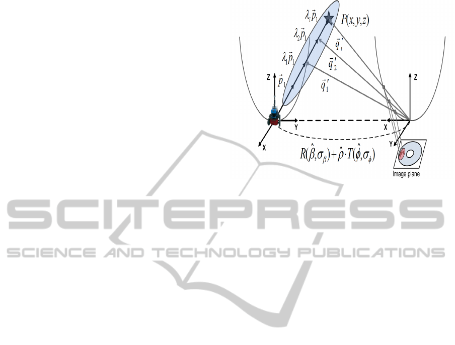
set of multi-scale points λ

for ~p

. This distribu-

tion considers a valid range for λ

according to the

predicted

ρ. Please note that the error of the current

estimation of the map has to be propagated along the

procedure. According to Kalman ﬁlter theory, the in-

novation is deﬁned as the difference between the pre-

dicted ˆz

and the real z

observation measurement:

(k + 1) = z

(k + 1) − ˆz

(k + 1|k) (7)

and the covariance of the innovation:

(k + 1) = H

(k)P(k +1|k)H

(k) + R

(k + 1) (8)

where H

(k) relates ¯x(k) and z

(k), P(k + 1|k) is a co-

variance matrix that expresses the uncertainty on the

estimation, and R(k) is the covariance of the gaussian

noise introduced in the process. In addition, S

(k + 1)

presents the following structure:

(k + 1) =



φβ

βφ



(9)

Next, since the predicted

E can be decomposed

in a rotation

R and a translation

T , we can transform

the distribution λ

into the second image reference

system, obtaining

. In order to propagate the er-

ror, we make use of (9) to redeﬁne the transforma-

tion through normal distributions, being R∼N(

β,σ

)

and T ∼N(

φ,σ

). This fact implies that

is a gaus-

sian distribution correlated with the current map un-

certainty. Once obtained

, they are projected into

the image plane of the second image, seen as crossed

points in Figure 4. This projection of the normal

multi-scale distribution deﬁnes a predicted area in

the omnidirectional image which is drawn in contin-

uous curve line. This area establishes the speciﬁc

image pixels where correspondences for ~p

must be

searched for. The shape of this area depends on the

error of the prediction, which is directly correlated

with the current uncertainty of the map estimation.

Dash lines represent the possible candidate points lo-

cated in the predicted area. Therefore, the problem

of matching is reduced to ﬁnding the correct corre-

sponding point for ~p

from those candidates inside

the predicted area by comparing their visual descrip-

tor, instead of searching for them at the whole image.

3.3 Computing the Transformation

Once a set of interest SURF points have been detected

and matched in two images it is necessary to retrieve

the relative angles β and φ. In the previous subsec-

tion was introduced the term

E for a predicted matrix

to ﬁnd valid correspondences. Now this set of cor-

responding points is known, the real E can be deter-

mined by directly solving (4). The essential matrix

Figure 3: Given a detected point ~p

in the ﬁrst image refer-

ence system, a point distribution is generated to obtain a set

of multi-scale points λ

. By using the Kalman prediction,

they can be transform to

in the second image reference

system through R∼N(

β,σ

), T ∼N(

φ,σ

) and

ρ. Finally

are projected into the image plane to determine a restricted

area where correspondences have to be found.

can be expressed as a speciﬁc rotation R and a trans-

lation T (up to a scale factor), where E = R · T

. The

use of a SV D decomposition makes able to retrieve

R and T . Following (Bunschoten and Krose, 2003;

Hartley and Zisserman, 2004) we obtain the relative

angles β and φ that deﬁne a planar motion between

images acquired from different poses. It is worth not-

ing that the motion is restricted to the XY plane, thus

only N = 4 correspondences are sufﬁcient to solve the

problem. Nevertheless we use higher number of cor-

respondences in order to get accurate solutions. No-

tice that now an external algorithm is not necessary

to reject false correspondences since we avoid them

through the restricted matching process, limited to

speciﬁc image area as recently explained.

4 RESULTS

We present three diferent experimental sets. Sec-

tion 4.1 ﬁrstly presents SLAM results to verify the

validity of this proposed approach of SLAM. In ad-

dition, it presents map building results when varying

the number of views that generate the map in order

to extract conclusions in the sense of the compact-

ness of the representation. Finally, we present results

of accuracy in the obtained map, use of computa-

tional resources and their variation with the number

of views that conform the map. To carry out these

experiments an indoor robot Pioneer P3-AT has been

used, which is equipped with a ﬁrewire 1280x960

View-basedSLAMusingOmnidirectionalImages

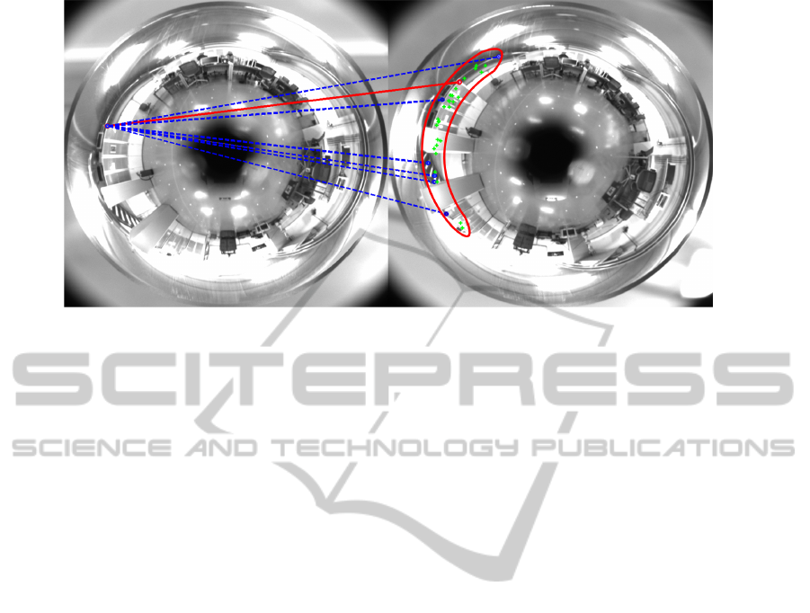
Figure 4: Correspondences for a speciﬁc point in the ﬁrst image are searched for in the predicted area, which is projected

into the second image. Crossed points represent the projection of the normal point distribution for the multi-scale points that

determine this area. Dash lines show the candidate points in the second image which are inside the predicted area. Continue

line represents the correct correspondence for a certain point in the ﬁrst image. Curve continue line shows the shape of the

predicted area.

camera and a hyperbolic mirror. The optical axis of

the camera is installed approximately perpendicular

to the ground plane, as described in Figure 1(a), in

consequence, a rotation of the robot corresponds to a

rotation of the image with respect to its central point.

Besides, in order to obtain a reference for compari-

son we use a SICK LMS range ﬁnder to generate a

ground truth (Stachniss et al., 2004) which provides a

resolution of 1m in position.

4.1 SLAM with Real Data

This section presents SLAM results of map build-

ing to validate the proposed approach. The robot is

guided through an ofﬁce-like environment of 32x35m

while it acquires omnidirectional images and laser

range data along the trajectory. Laser data is only used

to generate a ground truth for comparison. The robot

initiates the SLAM process by adding the ﬁrst view

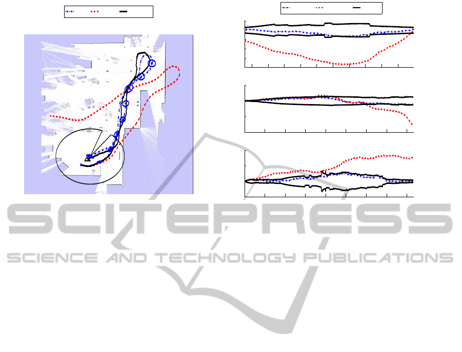
of the map at the origin, as indicated in Figure 5(a).

Next, it keeps on moving along the trajectory while

capturing omnidirectional images. The image at the

current robot pose is compared to the view in the map

looking for corresponding points in order to extract a

relative measurement of its position as explained in

Section 3. The evaluation of the similarity ratio (3)

is also computed, and in case this ratio drops below

R < 0.5, a new view is initialized at the current robot

position with an error ellipse. While the mapping con-

tinues, the current image is still being compared with

the rest of the views in the map. Figure 5(a) shows the

entire process where the robot ﬁnishes the navigation

going back to the origin. The dash-dotted line repre-

sents the solution obtained by the proposed approach,

indicating with crosses the points along the trajec-

tory where the robot decided to initiate new views

in the map and their uncertainty with error ellipses.

The continue line represents the ground truth whereas

the odometry is drawn with dash line. As it can be

observed, a map for an environment of 32x35m is

formed by a reduced set of N=9 views, thus leading to

a compact representation. Figure 5(b) compares the

errors for the estimated trajectory, the ground truth

and the odometry at every step of the trajectory. The

validity of the solution is conﬁrmed due to the ac-

complishment of the convergence required by every

SLAM scheme, since the solution error is inside the

2σ interval whereas the odometry error grows out of

bounds.

Once the proposed approach was validated, the

following experiments were carried out with the aim

of testing the compactness of the representation of

the environment. Another ofﬁce-like environment of

42x32m was chosen. In this case the threshold for

the similarity ratio R were varied in order to get dif-

ferent map representation for the same environment,

in terms of the number of views N that compose

the map. The procedure to build up the map fol-

lows the steps detailed in the ﬁrst experiment, and

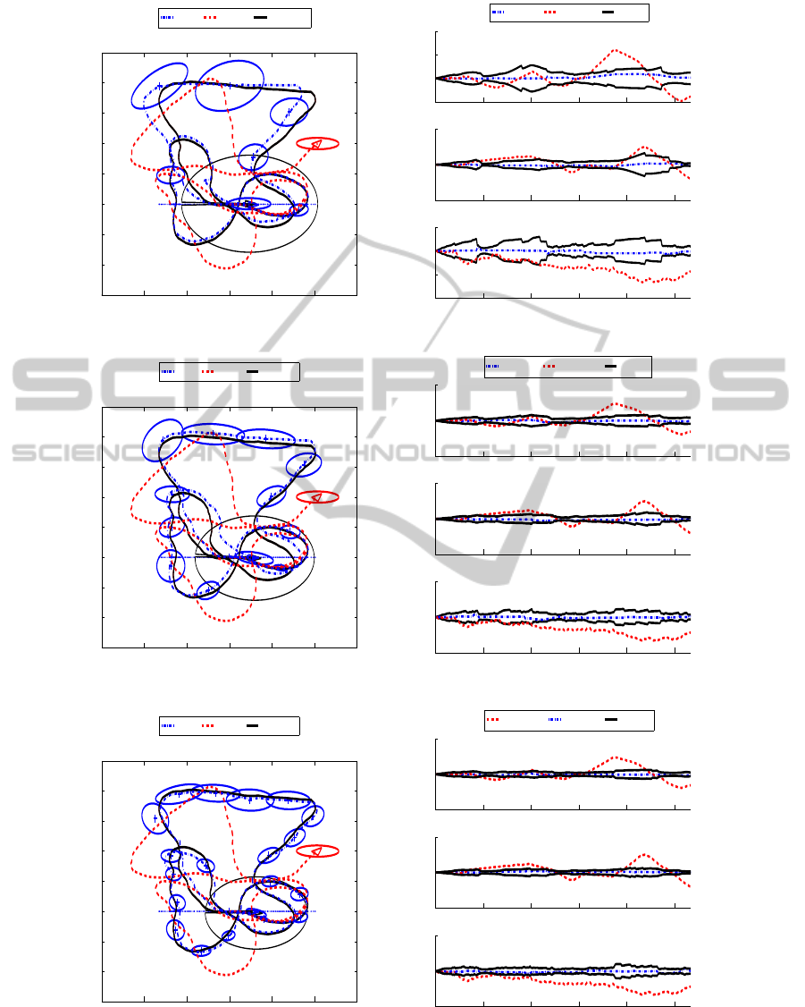
is depicted in Figure 6. Figures 6(a), 6(c), 6(e)

show different map versions for this environment with

N=7, N=12 and N=20 views respectively. Again, the

estimated solution is drawn in dash-dotted line, the

odometry in dash line, meanwhile the ground truth in

continuous line. View’s position are indicated with

crosses and their uncertainty with error ellipses. Fig-

ures 6(b), 6(d), 6(f), present the errors of the esti-

mated solution and the odometry versus 2σ intervals

ICINCO2012-9thInternationalConferenceonInformaticsinControl,AutomationandRobotics

3 9 12 15 18 21 24 27 32

X(m)

Y(m)

Map with N=9 views

Solution Odometry Ground truth

(a)

120 140 160 180 200 220 240 260 280 300

−1.5

−1

−0.5

0.5

Error X (m)

0 50 100 150 200 250 300 350 400

−0.5

0.5

Error θ (rad)

Map Step

0 50 100 150 200 250 300 350 400

−2

−1

Error Y (m)

Solution error Odometry error

2σ interval

(b)

Figure 5: Figure 5(a) presents results of SLAM using real data. The ﬁnal map is determined by N=9 views, which their

positions are represented with crosses and error ellipses. A laser-based occupancy map has been overlapped to compare with

the real shape of the environment. Figure 5(b) presents the solution and odometry error in X, Y and θ at each time step.

to test the convergence and validity of the approach

for each N-view map. All three estimations satisfy the

error requirements for the convergence of the SLAM

method, since the solution error is inside the 2σ inter-

val, however the odometry tends to diverge without

limit. According to this results, it should be noticed

that the higher values of N the lower resulting error

in the map. Nevertheless, with the lower value N=7

views, the resulting error is suitable to work in a re-

alistic SLAM problem in robotics. This fact reveals

the compactness of the representation. In some con-

text a compromise solution might be adopted when

choosing between N, error and obviously computa-

tional cost. Next paragraph analysis this issue.

The concept of compactness in the representation

of the map has been comﬁrmed by the previous re-

sults. It has been observed that lower values of N pro-

vide good results in terms of error. In addition more

experiments to obtain maps with different number of

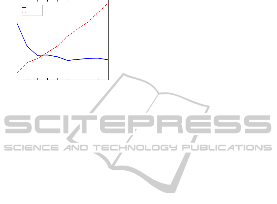
views N have been carried out. The results allow us to

analyze the computational cost in terms of the num-

ber of views N composing the map. In Figure 7 we

present these results, showing the RMS error in po-

sition and the time consumption, which reveal that

the error decreases when N increases. Consequently,

the accuracy of the estimation is higher since more

views are observed, however the computational cost

grows. That is the reason why a compromise solu-

tion has to be reached. Generally, SLAM algorithms

are real-time intended, so that the time is a limiting

factor. Despite this fact, the approach presented here

provides accurate results even using a reduced set of

views, which is a beneﬁt to consider when there is a

lack of computational resources.

5 CONCLUSIONS

In this paper it has been presented an approach to

the Simultaneous Localization and Mapping (SLAM)

problem using a single omnidirectional camera as a

visual sensor. We suggest a different representation

of the environment. In contrast to traditional 3D pose

estimation SLAM schemes, we only estimate the pose

and orientation of a set of omnidirectional images, re-

named views, as part of the map. A set of interest

points described by visual descriptors are associated

to each omnidirectional image so that a compact de-

scription of the environment is accomplished. Each

omnidirectional image allows the robot to compute its

localization in the image surroundings. A new match-

ing method is suggested to deal with the problem of

ﬁnding correspondences. Given two omnidirectional

images an a set of interest points for each one, we

model the relative error between them by means of

a gaussian distribution that correlates the current es-

timation error on the map to help us to compute a

more reliable transformation between images, com-

posed by a rotation and a translation (up to a scale

factor). This transformation allows to propose an ob-

servation model and to compute a trajectory over a

View-basedSLAMusingOmnidirectionalImages

0 7 14 21 28 35 42

MAP with N=7 views

X(m)

Y(m)

Solution Odometry Ground truth

(a)

0 50 100 150 200 250

−2

Error X (m)

0 50 100 150 200 250

−5

Error Y (m)

0 50 100 150 200 250

−2

−1

Error θ (rad)

Map Step

Solution error Odometry error

2σ interval

(b)

0 7 14 21 28 35 42

MAP with N=12 views

X(m)

Y(m)

Solution Odometry Ground truth

(c)

0 50 100 150 200 250

−5

Error X (m)

0 50 100 150 200 250

−5

Error Y (m)

0 50 100 150 200 250

−2

Error θ (rad)

Map Step

Solution error Odometry error

2σ interval

(d)

0 7 14 21 28 35 42

Map with N=20 views

X(m)

Y(m)

Solution Odometry Ground truth

(e)

0 50 100 150 200 250

−5

Error X (m)

0 50 100 150 200 250

−5

Error Y (m)

0 50 100 150 200 250

−2

Error θ (rad)

Map Step

Odometry error Solution error

2σ interval

(f)

Figure 6: Figures 6(a), 6(c), 6(e) present results of SLAM using real data obtaining different map representations of the

environment, formed by N=7, N=12 and N=20 views respectively. The position of the views is presented with error ellipses.

Figures 6(b), 6(d), 6(f), present the solution and odometry error in X, Y and θ at each time step for each N-view map.

ICINCO2012-9thInternationalConferenceonInformaticsinControl,AutomationandRobotics

10 20 30 40 50 60 70 80 90 100

0.2

0.4

0.6

0.8

RMS error (m)

Number of views N

10 20 30 40 50 60 70 80 90 100

0.02

0.04

0.06

0.08

Time (s)

RMS error (m)

Time (s)

Figure 7: RMS error (m) and time consumption (s) versus

the number of views N observed by the robot to compute its

pose inside different N-view maps.

map. We append map building results using an EKF-

based SLAM algorithm with real data acquisition us-

ing an indoor robot, to validate the SLAM approach.

In addition we have shown the compactness of the en-

vironment representation by building maps with dif-

ferent number of views. Finally we presented a set of

measurements to test the accuracy of the solution and

the time consumption as a function of the number of

views that conform the map.

ACKNOWLEDGEMENTS

This work has been supported by the Spanish govern-

ment through the project DPI2010-15308.

REFERENCES

Andrew J. Davison, A. J., Gonzalez Cid, Y., and Kita, N.

(2004). Improving data association in vision-based

SLAM. In Proc. of IFAC/EURON, Lisboa, Portugal.

Bay, H., Tuytelaars, T., and Van Gool, L. (2006). SURF:

Speeded up robust features. In Proc. of the ECCV,

Graz, Austria.

Bunschoten, R. and Krose, B. (2003). Visual odometry

from an omnidirectional vision system. In Proc. of

the ICRA, Taipei, Taiwan.

Civera, J., Davison, A. J., and Mart

ınez Montiel, J. M.

(2008). Inverse depth parametrization for monocular

slam. IEEE Trans. on Robotics.

Davison, A. J. and Murray, D. W. (2002). Simultaneous lo-

calisation and map-building using active vision. IEEE

Trans. on PAMI.

Gil, A., Martinez-Mozos, O., Ballesta, M., and Reinoso, O.

(2010a). A comparative evaluation of interest point

detectors and local descriptors for visual SLAM. Ma-

chine Vision and Applications.

Gil, A., Reinoso, O., Ballesta, M., Juli

a, M., and Pay

a, L.

(2010b). Estimation of visual maps with a robot net-

work equipped with vision sensors. Sensors.

Grisetti, G., Stachniss, C., Grzonka, S., and Burgard, W.

(2007). A tree parameterization for efﬁciently com-

puting maximum likelihood maps using gradient de-

scent. In Proc. of RSS, Atlanta, Georgia.

Harris, C. G. and Stephens, M. (1988). A combined corner

and edge detector. In Proc. of Alvey Vision Confer-

ence, Manchester, UK.

Hartley, R. and Zisserman, A. (2004). Multiple View Geom-

etry in Computer Vision. Cambridge University Press.

Jae-Hean, K. and Myung Jin, C. (2003). Slam with omni-

directional stereo vision sensor. In Proc. of the IROS,

Las Vegas (Nevada).

Joly, C. and Rives, P. (2010). Bearing-only SAM using a

minimal inverse depth parametrization. In Proc. of

ICINCO, Funchal, Madeira (Portugal).

Kawanishi, R., Yamashita, A., and Kaneko, T. (2008). Con-

struction of 3D environment model from an omni-

directional image sequence. In Proc. of the Asia Inter-

national Symposium on Mechatronics 2008, Sapporo,

Japan.

Montemerlo, M., Thrun, S., Koller, D., and Wegbreit, B.

(2002). FastSLAM: a factored solution to the simul-

taneous localization and mapping problem. In Proc. of

the 18th national conference on Artiﬁcial Intelligence,

Edmonton, Canada.

Murillo, A. C., Guerrero, J. J., and Sag

es, C. (2007). SURF

features for efﬁcient robot localization with omnidi-

rectional images. In Proc. of the ICRA, San Diego,

USA.

Nister, D. (2003). An efcient solution to the ﬁve-point rela-

tive pose problem. In Proc. of the IEEE CVPR, Madi-

son, USA.

Scaramuzza, D. (2011). Performance evaluation of 1-point

RANSAC visual odometry. Journal of Field Robotics.

Scaramuzza, D., Fraundorfer, F., and Siegwart, R. (2009).

Real-time monocular visual odometry for on-road ve-

hicles with 1-point RANSAC. In Proc. of the ICRA,

Kobe, Japan.

Stachniss, C., Grisetti, G., Haehnel, D., and Burgard, W.

(2004). Improved Rao-Blackwellized mapping by

adaptive sampling and active loop-closure. In Proc.

of the SOAVE, Ilmenau, Germany.

Stewenius, H., Engels, C., and Nister, D. (2006). Recent de-

velopments on direct relative orientation. ISPRS Jour-

nal of Photogrammetry and Remote Sensing.

View-basedSLAMusingOmnidirectionalImages