Performance Shaping through Cost Cumulants and Neural

Networks-based Series Expansion

Bei Kang, Chukwuemeka Aduba and Chang-Hee Won

Department of Electrical and Computer Engineering, Temple University, Philadelphia, PA 19122, U.S.A.

Keywords:

Statistical Optimal Control, Cumulant Minimization, Neural Networks, Cost Cumulants, Performance

Shaping.

Abstract:

The performance shaping method is addressed as a statistical optimal control problem. In statistical control,

we shape the distribution of the cost function by minimizing n-th order cost cumulants. The n-th cost cumu-

lant, Hamilton-Jacobi-Bellman (HJB) equation is derived as the necessary condition for the optimality. The

proposed method provides an approach to control a higher order cost cumulant for stochastic systems, and

generalizes the traditional linear-quadratic-Gaussian and Risk-Sensitive control methods. This allows the cost

performance shaping via the cost cumulants. Moreover, the solution of general n-th cost cumulant control is

provided by numerically solving the HJB equations using neural network method. The results of this paper

are demonstrated through a satellite attitude control example.

1 INTRODUCTION

We shape the performance of the system through the

statistical properties of the cost function. In linear-

quadratic-Gaussian (LQG) control, the performance

is optimized by minimizing the mean of the cost func-

tion (Fleming and Rishel, 1975). In statistical opti-

mal control, we minimize any cost cumulant to im-

prove the performance of the system. So far the ﬁrst

mean (LQG) and denumerable sum of all the cumu-

lants (risk-sensitive) of the cost function are inves-

tigated (Lim and Zhou, 2001). However, there are

other statistical parameters that we can vary to shape

the performance. This is achieved by minimizing n-th

cost cumulants. The study of cost control cumulant

was initiated by (Sain, 1966). The authors extended

the theory of cost cumulant control to third and fourth

cumulants for a nonlinear system with nonquadratic

cost and derived the corresponding HJB equations

(Won et al., 2010). HJB equation was derive, but

the solution was not determined. In fact, most HJB

equations do not have analytical solutions except for

the special cases of linear systems with quadratic cost

functions. Thus, numerical approximate methods are

needed to solve HJB equation. For the ﬁrst two cu-

mulant case, we solved the HJB equation using neu-

ral networks in (Kang and Won, 2010). In this paper,

we extend this result to n-th cumulants. This is not a

simple extension of the results in (Won et al., 2010).

There, we developed a procedure to solve higher or-

der cost cumulant problem using the results of the mo-

ments. In this paper, we use induction to derive n-th

cumulant HJB equation, which was not a trivial task.

This n-th cumulant HJB equation corresponds to the

performance shaping idea. Then we solve this HJB

equation using a neural network method.

A power series expansion to approximate the

value function for an inﬁnite-time horizon determin-

istic system was given in (Alberkht, 1961). Apply-

ing Galerkin approximate method to solve the gen-

eralized Hamilton-Jacobi-Bellman (GHJB) was given

in (Beard et al., 1997). (Chen et al., 2007) proposed

using neural network methods to solve the optimal

control problem of a nonlinear ﬁnite time system. If

we deﬁne the weighting and the basis functions as

polynomials, the neural network is in fact equivalent

to power series expansion in that we use coefﬁcients

of the power expansion as the weights in neural net-

works. However, neural network method has the po-

tential to be more than simple power series expansion

by adding additional layers of neurons. In this work,

we extend the system dynamics of (Chen et al., 2007)

to stochastic systems. Then we solve the HJB equa-

tions for the n-th cost cumulant control problem using

neural network approximation method.

Section 2 states the problem and deﬁnes the nota-

tions used in this paper. Section 3 develops the HJB

equations for the n-th cost cumulant control of the

196

Kang B., Aduba C. and Won C..

Performance Shaping through Cost Cumulants and Neural Networks-based Series Expansion.

DOI: 10.5220/0004032101960201

In Proceedings of the 9th International Conference on Informatics in Control, Automation and Robotics (ICINCO-2012), pages 196-201

ISBN: 978-989-8565-21-1

 2012 SCITEPRESS (Science and Technology Publications, Lda.)

system. The induction is utilized in the derivation. In

order to solve the statistical optimal control problem,

we use neural network approximations for HJB equa-

tions in Section 4. The simulation results for the satel-

lite attitude control application is presented in Section

5. Finally conclusions are given in the last section.

2 PROBLEM FORMULATION

Consider a stochastic differential equation:

dx(t) = f(t, x(t), u(t))dt + σ(t, x(t))dw(t),

(1)

where t ∈ [t

], x(t

) = x

, x(t) ∈ R

, u(t) ∈U ⊂ R

and dw(t) is a Gaussian random process of dimension

d with zero mean and covariance of W(t)dt. The sys-

tem control is given as

u(t) = k(t, x(t)),t ∈ T.

(2)

The system cost function is given as:

J(t, x(t);k) = ψ(x(t

))



l(s, x(s)) + k

′

(s, x(s))Rk(s, x(s))



ds,

(3)

where ψ(x(t

)) is the terminal cost, l(s, x(s)) is a pos-

itive deﬁnite function, R is the positive deﬁnite matrix.

The goal is to ﬁnd an optimal controller for system (1)

which minimizes the n-th cumulant of the cost func-

tion (3), such that V

(t, x, k(t, x)) = min

k∈K

(t, x, k)}.

We now introduce a backward evolution operator

O (k), deﬁned by

O (k) =

∂

∂t

∑

i=0

(t, x, k(t, x))

∂

∂x

∑

i, j=1



σ(t, x)W(t)σ

′

(t, x)



i, j

∂

∂x

Then the n-th cumulant of cost function, we in-

troduce the n-th moments of cost function which is

deﬁned as:

(t, x, k(t, x)) = E

(t, x, k(t, x))



x(t) = x

Next, we introduce some deﬁnitions,

Deﬁnition 2.1. A function M

: Q

→ R

is an

admissible j-th moment cost function if there ex-

ists an admissible control law k such that M

(t, x) =



(t, x, k(t, x))



for t ∈ T, x ∈ R

Deﬁnition 2.2. The admissible moment cost func-

tions M

, ..., M

deﬁnes a class of control laws K

such that for each k ∈ K

, M

, ..., M

satisfy Deﬁni-

tion 2.1.

Deﬁnition 2.3. A function V

: Q

→ R

is an admis-

sible j-th cumulant cost function if there exists an ad-

missible control laws k such that V

(t, x) = V

(t, x, k).

Now, we mathematically formulate the statistical

optimal control problem as follows. Under the as-

sumption that M

, ..., M

n−1

exist and are admissi-

ble, we ﬁnd an optimal control k

∗

∈ K

such that

∗

(t, x) = V

(t, x, k

∗

) satisﬁes V

∗

(t, x) ≤ V

(t, x, k) for

all k(t, x) ∈ K

(t, x).

The n-th cumulant of the cost function is given by

the following recursion formula (Smith, 1995), where

we suppress the arguments for the sake of brevity.

= M

−

n−2

∑

i=0

(n− 1)!

i!(n− 1− i)!

n−1−i

i+1

(4)

It is shown in (4) that the n-th order cumulant

can be calculated from the n-th order moment and the

lower order moments and cumulants. In the next sec-

tion, the above deﬁnitions and formulas will be used

to derive the HJB equations for the n-th order cumu-

lant minimization.

3 n-th CUMULANT HJB EQ.

Before we derive the n-th cumulant HJB equation,

we introduce the n-th moment HJB equation. (Sain,

1967) derived the n-th moment HJB equation given in

recursive form,

O (k)[M

(t, x, k)] + nM

n−1

(t, x, k)L(t, x, k) = 0

(5)

Using (5) and the Deﬁnition 2.1, we have the fol-

lowing theorem which gives the necessary condition

for the optimality. Consider on open set Q

⊂ (

Theorem 3.1. Let M

(t, x) ∈ C

1,2

)∩C(

) be the

j-th admissible moment cost function, assume the ex-

istence of an optimal controller k

∗

∈ K

such that

∗

(t, x) = M

(t, x, k

∗

) = min

k∈K



(t, x, k)



then k

∗

and M

∗

satisfy the following HJB equation,

O (k)



∗

(t, x)



+ jM

j−1

(t, x)L(t, x, k

∗

) = 0,

(6)

for t ∈ T, x ∈ R

and the terminal condition is given

as M

∗

, x) = ψ(x(t

)).

Proof: See (Won et al., 2010).

The following Lemmas are used to obtain the n-th

cumulant HJB equation.

Lemma 3.1. Consider two functions M

(t, x), V

(t, x)

∈ C

1,2

(Q) ∩C(

Q), where i and j are non-negative in-

tegers, then

O (k)[M

(t, x)V

(t, x)]

= O (k)[M

(t, x)]V

(t, x) + M

(t, x)O (k)[V

(t, x)]



∂M

(t, x)

∂x



′

σ(t, x)Wσ(t, x)

′



∂V

(t, x)

∂x



PerformanceShapingthroughCostCumulantsandNeuralNetworks-basedSeriesExpansion

197

Lemma 3.2. Let V

(t, x), ..., V

k−1

(t, x) ∈ C

1,2

(Q) ∩

Q) be admissible cost cumulant functions, then

k−1

∑

s=1

s!(k− s)!



∂V

∂x



′

σWσ

′



∂V

k−s

∂x



k−2

∑

i=0

(k− 1)!

i!(k− 1− i)!



∂V

k−1−i

∂x



′

σWσ

′



∂V

i+1

∂x



Proof: Omitted for brevity.

The main result of this paper is given in the fol-

lowing theorem. We use induction to prove the gen-

eral n-th cumulant optimal control.

Theorem 3.2. (n-th cumulant HJB equation) Let

(t, x),V

(t, x), . . . ,V

n−1

(t, x) ∈ C

1,2

) ∩C(

) be

an admissible cumulant cost function for the con-

trol. Assume the existence of an optimal control law

∗

∈ K

and an optimal value function V

∗

(t, x) ∈

1,2

) ∩ C(

). Then the minimal n-th cumu-

lant cost function V

∗

(t, x) satisﬁes the following HJB

equation,

0 = min

k∈K

(

O (k)[V

∗

]

n−1

∑

s=1

s!(n− s)!



∂V

∂x



′

σWσ

′



∂V

n−s

∂x



)

(7)

for (t, x) ∈

, with the terminal conditionV

∗

, x) =

Proof: The mathematical induction method is used

here to prove the theorem. We proved that when n=2,

the second cost cumulant HJB equation satisﬁes (1).

The third and fourth cumulant cases were proved in

(Won et al., 2010). Thus, we assume that this theorem

holds for the second, third and (n-1)-th cumulant case.

We will show that the theorem also holds for the n-th

cumulant case. Henceforth, the arguments of M and

V are suppressed for brevity.

Let V

∗

be in the class of C

1,2

(Q) ∩ C(

Q). Apply

the backward evolution operator O (k) to the recursive

formula (4), we have

0 = O (k)[V

∗

] − O (k)[M

]

n−2

∑

i=0

(n− 1)!

i!(n− 1− i)!

O (k)[M

n−1−i

i+1

(8)

From Theorem 3.1, we have

O (k)[M

] + nM

n−1

L = 0.

(9)

Then, from Lemma 3.1, and letting i = n − 1− i, j=

i+ 1, we obtain

O (k)[M

n−1−i

i+1

] = O (k)[M

n−1−i

i+1

+ M

n−1−i

O (k)[V

i+1

] +



∂M

n−1−i

∂x



′

σWσ

′



∂V

i+1

∂x



(10)

Substitute (9), (10) into (8), and we have

0 = O (k)[V

∗

] + nM

n−1

n−2

∑

i=0

(n− 1)!

i!(n− 1− i)!

O (k)[M

n−1−i

i+1

+ M

n−1−i

O (k)[V

i+1

] +



∂M

n−1−i

∂x



′

σWσ

′



∂V

i+1

∂x



(11)

Use (9) again for O (k)[M

n−1−i

] in (11) results in

0 = O (k)[V

∗

] + nM

n−1

n−2

∑

i=0

(n− 1)!

i!(n− 1− i)!

− (n− 1− i)M

n−2−i

i+1

+ M

n−1−i

O (k) [V

i+1

] +



∂M

n−1−i

∂x



′

σWσ

′



∂V

i+1

∂x



(12)

Using the formula in (Stuart and Ord, 1987),

∂M

∂V

j!(i− j)!

i− j

then

∂M

n−1−i

∂x

n−1−i

∑

j=1

(n− 1− i)!

j!(n− 1− i− j)!

n−1−i− j

∂V

∂x

Thus, using the assumption that the theorem holds,

from second order to (n− 1)-th order cumulant case,

(12) becomes

0 = O (k)[V

∗

] −

n−2

∑

i=1

(n− 1)!

i!(n− 1− i)!

n−1−i

i−1

∑

j=0

j!(i− j)!



∂V

i− j

∂x



′

σWσ

′



∂V

j+1

∂x



n−2

∑

i=0

(n− 1)!

i!(n− 1− i)!

n−1−i

∑

j=1

(n− 1− i)!

j!(n− 1− i− j)!

n−1−i− j



∂V

∂x



′

σWσ

′



∂V

i+1

∂x



(13)

From (13), we notice that both the second and third

term on the right hand side contain the moment from

}, where x = 1, 2, .. . , n − 2. Therefore, it is

feasible to combine two summations with respect to

and simplify the equation. For derivation conve-

nience, we use p and q instead of i and j within the

bracket of the second term of (13),

n−1−i

i−1

∑

j=0

j!(i− j)!



∂V

i− j

∂x



′

σWσ

′



∂V

j+1

∂x



to distinguish the notations of the second and third

term in (13). Note that the notations p, q and i, j are

indeed equivalent. Therefore, (13) is rewritten as

ICINCO2012-9thInternationalConferenceonInformaticsinControl,AutomationandRobotics

198

O (k)[V

∗

] −

n−2

∑

p=1

(n− 1)!

p!(n− 1− p)!

n−1−p

p−1

∑

q=0

q!(p− q)!



∂V

p−q

∂x



′

σWσ

′



∂V

q+1

∂x



n−2

∑

i=0

(n− 1)!

i!(n− 1− i)!

n−2−i

∑

j=1

(n− 1− i)!

j!(n− 1− i− j)!

n−1−i− j



∂V

∂x



′

σWσ

′



∂V

i+1

∂x



n−2

∑

i=0

(n− 1)!

i!(n− 1− i)!



∂V

n−1−i

∂x



′

σWσ

′



∂V

i+1

∂x



= 0.

(14)

Now, let us focus on the second and third terms of

(14). We consider the second and third terms as func-

tions with respect to M

. We will compare the coef-

ﬁcients of the same M

on second and third terms,

i.e when M

n−1−p

= M

n−1−i− j

. When k − 1 − p =

k− 1− i− j, then p = i+ j, then we will determine the

corresponding coefﬁcients associated with M

n−1−p

n−1−i− j

via the following procedure. In the second

term of (14), the coefﬁcient associated with M

n−1−p

−

p−1

∑

q=0

(n− 1)!

q!(n− 1− p)!(p − q)!



∂V

p−q

∂x



′

σWσ

′



∂V

q+1

∂x



n−1−p

(15)

For the third term in (14) because p = i+j, then for

each p in [1, n-2], there are combinations of i and j,

such that the summation of which are equal to p such

as p=0+p, p=1+(p-1), ...and p=(p-1)+1. Because

the range for index i is i = 0, 1, 2, ..., p-1, when we

look for the coefﬁcient of M

n−1−i− j

when M

n−1−i− j

n−1−p

, we must ﬁnd summation of the coefﬁcient of

n−1−i− j

for all combinations of i and j. Therefore,

the corresponding coefﬁcient is

i=p−1

∑

i=0, j=p=i

n−1−i− j

where C

n−1−i− j

is the coefﬁcient for each i and j

which lead to the same k-1-i-j. Substitute p = i +

j, i = 0, 1, 2, ..., p-1, j = p-i back to the third term of

(14), then the coefﬁcient associated with M

n−1−i− j

p−1

∑

i=0

(n− 1)!M

n−1−p

i!(n− 1− i)!

(n− 1− i)!

(p− i)!(n − 1 − p)!



∂V

p−i

∂x



′

σWσ

′



∂V

i+1

∂x



p−1

∑

i=0

(n− 1)!

i!(n− 1− p)!(p − i)!



∂V

p−i

∂x



′

σWσ

′



∂V

i+1

∂x



n−1−p

(16)

Compare (15) and (16), we notice that since p is

equivalent to i and q is equivalent to j, it is obvi-

ous that they have exactly format except for the signs.

Thus they will cancel with each other when they are

summed up. Therefore, the summation of the sec-

ond and third term on (14) will be zero. Then we

apply Theorem 3.1, (14) becomes (7). The theorem is

proved. 

4 NEURAL NETWORK APPROX.

Neural network method based on series expansion ap-

proximate concept for HJB equations is applied to

solve the value function of the HJB equations gen-

erated in the Section 3.

In our neural network approach, several neural

network input function are multiplied by their cor-

responding weights and then summed up to pro-

duce output which is the approximated value func-

tion. In this paper, polynomial series expansion

(x) = {δ

(x), δ

(x), . . . , δ

(x)}

′

is the neural net-

work input function while the weights of the series ex-

pansion is w

(t) = {w

(t), w

(t), . . . , w

(t)}

′

. These

weights are time-dependent. The n-th cumulant value

function is represented as V

∗

(x,t) = w

′

(t)

(x) =

∑

i=1

′

(t)δ

(x). The subscript L in the value func-

tion represents the order of the polynomial series. The

higher the order of the series, the closer the approxi-

mate value gets to the real value.

In Theorem 3.2, the HJB equation for the n-th

cumulant case is given. We need to solve this HJB

equation to ﬁnd the optimal controller. The optimal

controller k

∗

for the n-th cumulant case has the form.

∗

= −

−1

′



∂V

∂x

+ γ

∂V

∂x

. . . + γ

∂V

∗

∂x



(17)

with terminal condition V

∗

, x) = 0 where

, γ

, . . . , γ

are the Lagrange multipliers. From

(1), we assume that

f(t, x(t), k(t, x(t))) = g(t, x) + B(t, x)k(t, x),

where the matrices R(t) > 0, B(t, x) are continuous

real matrices. We substitute k

∗

back into the HJB

equation from the ﬁrst to n-th cumulant cases, then

use neural network series expansion to approximate

each HJB equation. Assuming terminal conditions for

the value function V

, . . . ,V

are zero.

PerformanceShapingthroughCostCumulantsandNeuralNetworks-basedSeriesExpansion

199

Then the neural network approximations are used.

We approximage V

by V

(x,t) = w

′

(t)

(x), V

by V

(x,t) = w

′

(t)

(x), etc. We obtain differen-

tial equations for the weigths. The n-th order one is

given as an example.

(t) =

− h

(x),

(x)i

−1

Ω

h∇

(x)g(x),

(x)i

Ω

¯w

(t)

(x),

(x)i

−1

Ω

¯w

(t)

∑

i=2

(x),

(x)i

−1

Ω

¯w

(t)

−

n−1

∑

i=1

i!(n− i)!

(x),

(x)i

−1

Ω

¯w

(n−i)L

−

(x),

(x)i

−1

Ω

¯w

(18)

The terminal conditions ¯w

),..., ¯w

) are

assumed zero and the quantities A

, B

, C

, F

and

are deﬁned as follows,

∑

s=1

(t)h∇

(x)BR

−1

′

∇

(x)

(x)i

Ω

∑

s=1

(t)h∇

(x)BR

−1

′

∇

(x)

(x)i

Ω

= htr



σWσ

′

∇



∇

′

(x) ¯w

(t)



(x)i

Ω

∑

s=1

(t)h∇

(n−i)L

(x)σWσ

′

∇

(x)

(x)i

Ω

= htr



σWσ

′

∇



∇

′

(x) ¯w

(t)



(x)i

Ω

To solve the n-th cumulant neural network equation,

we need to simultaneously solve all the n-th cumulant

equation by converting the PDEs to neural network

ODEs. Then, we solve the approximated ODEs with

the corresponding Lagrange multipliers γ

, γ

5 SIMULATION

In this section, we will use the neural network to cal-

culate the ﬁrst, second third and fourth cumulant opti-

mal control for a satellite attitude control application

studied in (Won, 1999). This is a linear system with

quadratic cost function. We deﬁne the state variables

as follows: ¯x = [x

, x

] =

[φ, θ, ψ, ω

, ω

, Ω

]. φ, ψ and θ are

the roll, yaw and pitch Euler angles of the satellite.

, ω

and ω

are the angular velocities of the satel-

lite. Ω

, Ω

and Ω

are the reaction wheel ve-

locities. We consider the fourth cumulant control

and analyze the system state space form and derive

the HJB equations for the fourth cumulant control.

Let V

(x,t) = w

′

(t)

(x) to approximate V

(x,t),

(x,t) = w

′

(t)

(x) to approximate V

(x,t), etc.

The basis function

(x) is chosen from the expan-

sion of a polynomial generating function (x

+ x

)

which contains

55 elements. Thus, the weights to be determined

are deﬁned as w

(t) = {w

, w

, . . . , w

}, w

(t) =

, w

, . . . , w

110

}, w

(t) = {w

111

, w

112

, . . . , w

165

(t) = {w

166

, w

167

, . . . , w

220

}. Using neural net-

work method, we solve for the approximatedV

(x,t),

(x,t), V

(x,t) and V

(x,t) .

Here we simulate the ﬁrst four cost cumulant con-

trol, i.e n = 4. Because we use Lagrange multiplier

method to derive the second, third and fourth cost cu-

mulant HJB equations, we solve the HJB equations

by assigning different values for the Lagrange multi-

pliers γ

, γ

and γ

. In all simulation, we ﬁx γ

= γ

= 0.001, while γ

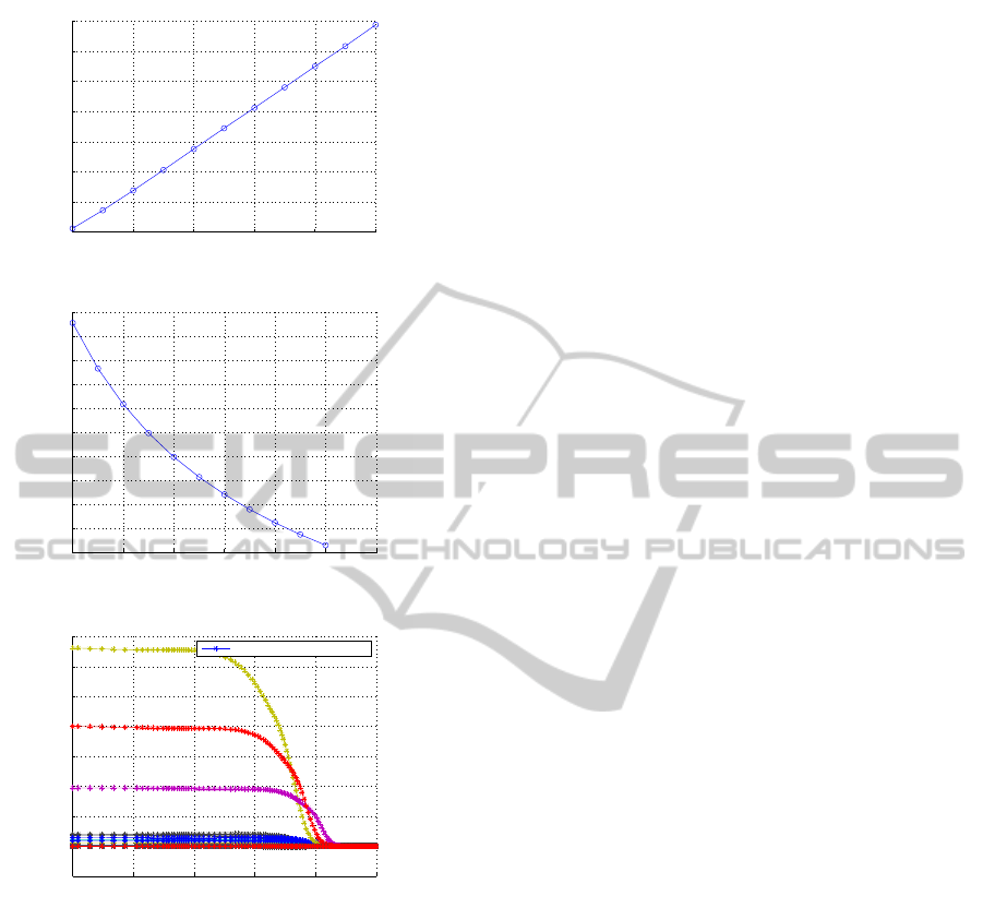
vary from 0 to 0.0001. In Fig. 1(a),

we observe that ﬁrst cumulant V

increases with in-

creases in γ

and the smallest V

is obtained when γ

is 0. For brevity we did not show second and third cu-

mulant value functions as a function of gamma

. The

second cumulant V

decreases with with increases in

and reaches a minimum when γ

= 0.0001. This is

related to the variance of the cost function. It is ob-

served thatV

decreases with increases in γ

. Fig. 1(b)

shows the fourth cumulant V

as γ

varies in value. It

is observed V

decreases with increases in γ

. Fig.

1(c) shows that the neural network weights converge

to constants when integrated backward in time.

Depending on the desired statistical properties of

the cost function, the engineer will choose the appro-

priate Lagrange multiplier values. In the satellite at-

titude control case, the mean and the variance are the

important factors. Thus γ

equal to 0.0001 is a good

choice. From the value functions, the corresponding

optimal controller k

∗

is determined by substituting V

, V

and V

back to the following equation,

∗

= −

−1

′



∂V

∂x

+ γ

∂V

∂x

+ γ

∂V

∂x

+ γ

∂V

∗

∂x



(19)

The optimal controller k

∗

(t,x) is the minimal

fourth cumulant controller. Similarly, the minimal

ﬁrst cumulant controller (LQG control) is found by

letting γ

= γ

= 0. Following similar approach,

we can determine higher order cumulant optimal con-

troller.

6 CONCLUSIONS

In this paper, we studied the statistical optimal control

ICINCO2012-9thInternationalConferenceonInformaticsinControl,AutomationandRobotics

200

0 0.2 0.4 0.6 0.8 1

x 10

−4

9600

9700

9800

9900

10000

10100

10200

10300

First Cumulant, γ

from 0 to 0.0001, γ

= γ

= 0.001

−Cost Cumulant Value Function

(a) V1

0 0.2 0.4 0.6 0.8 1 1.2

x 10

−4

2.6

2.8

3.2

3.4

3.6

3.8

4.2

4.4

4.6

x 10

Fourth Cumulant, γ

from 0 to 0.0001, γ

= γ

= 0.001

−Cost Cumulant Value Function

(b) V4

0 20 40 60 80 100

−1

x 10

192 Neural network weights

Time(sec)

Neural Network Weights

Neural Network Weights 1 to 192

Figure 1: Value Functions and Neural Network Weights.

problem. Statistical control shapes the cost cumulants

to improve the performance of the controller. We de-

rived the necessary condition for minimizing the n-th

cost cumulant for a givensystem. By shaping the den-

sity function, we improve the system performance.

The HJB equation for the n-th cumulant minimiza-

tion is derived. The optimal controller for the n-th

cumulant minimization problems is found by solving

the corresponding HJB equations. The n-th cumulant

HJB equation is numerically solved using neural net-

work method. In the satellite attitude control problem,

the performance is shaped using the Lagrange multi-

plier, which decreased the fourth cumulant, while the

ﬁrst cumulant increased.

ACKNOWLEDGEMENTS

This material is based upon work supported in part by

the National Science Foundation AIS Grant, ECCS-

0969430.

REFERENCES

Alberkht, E. G. (1961). On the Optimal Stabilization of

Nonlinear Systems. PMM - Journal of Applied Math-

ematics and Mechanics, 25:1254–1266.

Beard, R., Saridis, G., and Wen, J. (1997). Sufﬁcient Con-

ditions for the Convergence of Galerkin Approxima-

tions to the Hamilton-Jacobi Equation. Automatica,

33(12):2159–2177.

Chen, T., Lewis, F. L., and Abu-Khalaf, M. (2007). A Neu-

ral Network Solution for Fixed-Final Time Optimal

Control of Nonlinear Systems. Automatica, 43:482–

490.

Fleming, W. H. and Rishel, R. W. (1975). Determinis-

tic and Stochastic Optimal Control. Springer-Verlag,

New York.

Kang, B. and Won, C. (2010). Nonlinear Second Cost

Cumulant Control using Hamilton-Jacobi-Bellman

Equation and Neural Network Approximation. In

Proc. of the American Control Conference, Baltimore,

MD.

Lim, A. E. and Zhou, X. Y. (2001). Risk-Sensitive Control

with HARA Utility. IEEE Transactions on Automatic

Control, 46(4):563–578.

Sain, M. K. (1966). Control of Linear Systems According

to the Minimal Variance Criterion—A New Approach

to the Disturbance Problem. IEEE Transactions on

Automatic Control, AC-11(1):118–122.

Sain, M. K. (1967). Performance Moment Recursions, with

Application to Equalizer Control Laws. In Proc. of

Annual Allerton Conference on Circuit and System

Theory, Monticello, IL.

Smith, P. J. (1995). A Recursive Formulation of the Old

Problem of Obtaining Moments from Cumulants and

Vice Versa. The American Statistician, 49(2):217–

218.

Stuart, A. and Ord, J. K. (1987). Kendall’s Advanced The-

ory of Statistics:Distribution Theory. Oxford Univer-

sity Press, New York, 5th edition.

Won, C., Diersing, R. W., and Kang, B. (2010). Sta-

tistical Control of Control-Afﬁne Nonlinear Systems

with Nonquadratic Cost Function:HJB and Veriﬁca-

tion Theorems. Automatica, 46(10):1636–1645.

Won, C.-H. (1999). Comparative Study of Various Con-

trol Methods for Attitude Control of a LEO Satellite.

Aerospace Science and Technology, 3(5):323–333.

PerformanceShapingthroughCostCumulantsandNeuralNetworks-basedSeriesExpansion

201