Identiﬁcation of Polytopic Models for a Linear Parameter-varying

System Performed on a Vehicle

Raluca Liacu, Dominique Beauvois and Emmanuel Godoy

Automatic Departement, Supelec Sciences of Systems (E3S), Paris, France

Keywords:

LPV Model Identiﬁcation, Polytopic Model, Automotive Identiﬁcation.

Abstract:

This paper deals with the parameter identiﬁcation of continuous time polytopic models for a linear parameter-

varying system (LPV). A continuous-time nonlinear identiﬁcation approach is presented, a mix between a

local approach and a global one is introduced in order to identify a LPV model for the lateral comportement of

a vehicle. The proposed approach is based on the prediction error method for LTI systems, which is modiﬁed

to take into account polytopic models and regularization terms. Using experimental data, different parameter-

varying structures, explaining the lateral behavior of the vehicle, were identiﬁed by the proposed method

considering the velocity as the scheduling parameter.

1 INTRODUCTION

In the last years, the ﬁeld of Linear Parameter-Varying

(LPV) systems has drawn a great attention in the in-

dustrial control with a growing number of successful

applications.

Interest for such models is largely justiﬁed by the

ability they offer to design gain scheduling control as-

suming guaranteed stability for nonlinear systems.

Classical LPV models are formed using polytopic

structures constructed by a linear combination of mul-

tiple LTI models obtained at each operating point.

The operating points are chosen from the range of

the scheduling parameter. Such an experimental ap-

proach is not always feasible because of difﬁculties

with experiments (safety, cost, duration...). For our

application, identiﬁcation of the lateral behavior of

the vehicle, this leads us to an one-shot estimation of

different LTI models based on a single record with a

varying scheduling parameter.

Two situations were considered for the LTI mod-

els: the ﬁrst situation assumes that we do not know

how the model depends on the scheduling parameter.

For this assumption we have created a fully parame-

terized structure which is suitable in any situation. In

the second case, we consider that the dependence of

the model on the scheduling parameter is known and

the developed structure is based on the bicycle model.

In this paper the polytopic model is found using

the prediction error method based on a quadratic cri-

terion error in the time domain, leading to a global,

nonlinear optimization approach.

This paper presents adaptations of the standard

prediction error method to the proposed polytopic

structures.

The paper is organized as follows: in section 2 the

polytopic model and the two LPV model structures

are presented. Section 3 discusses the prediction error

method for polytopic models. In section 4 the identi-

ﬁcation background is presented based on a real data

experiment. In section 5 the results are analyzed and

the two models for the lateral behavior of a vehicle

are validated.

2 POLYTOPIC MODEL

A parameter varying system is considered. It is mod-

eled in the state space and is described by the follow-

ing equations:











dx(t)

= A(p(t),ξ(p))(x(t)) + B(p(t),ξ(p))u(t)

+K(p(t), ξ(p))e(t)

y(t) = C(p(t), ξ(p))(x(t)) + D(p(t), ξ(p))u(t)

+e(t)

(1)

where x(t), y(t), u(t), e(t) represent the state variable,

the output, the input and a stochastic white noise re-

spectively. p(t) is a measurable scheduling parame-

ter with respect to time. ξ(p) is the parameter vector

which is varying with respect to p.

470

Liacu R., Beauvois D. and Godoy E..

Identiﬁcation of Polytopic Models for a Linear Parameter-varying System Performed on a Vehicle.

DOI: 10.5220/0004032504700475

In Proceedings of the 9th International Conference on Informatics in Control, Automation and Robotics (ICINCO-2012), pages 470-475

ISBN: 978-989-8565-21-1

 2012 SCITEPRESS (Science and Technology Publications, Lda.)

2.1 General Structure of a Polytopic

Model

In this section the polytopic model for the considered

system is presented. For each value p

of p, the sys-

tem is characterized by an LTI structure (A

,ξ

),...,

,ξ

), ξ

= ξ(p

)), named the i

local LTI model.

A polytopic structure is formed considering a state

space representation given by:

(p,θ) =

∑

i=1

(p)A

,ξ

)

(p,θ) =

∑

i=1

(p)B

,ξ

)

(p,θ) =

∑

i=1

(p)C

,ξ

)

(p,θ) =

∑

i=1

(p)D

,ξ

)

(p,θ) =

∑

i=1

(p)K

,ξ

)

(2)

with θ = [ξ

... ξ

] and w

(p) being the weighting

functions satisfying the following relations :

(p) ≥ 0,∀i,

∑

i=1

(p) = 1

(3)

where r is the number of operating points chosen to

represent the model and p

is the i-th operating point

of the scheduled signal. Figure 1 shows the weighting

functions chosen as triangular functions.

The objective of this paper is the following: us-

ing the input, output and the scheduled signal data

(u,y, p) measured from the original system, estimate

the vector θ in the polytopic form (2) so that the pre-

dicted output of the model denoted by ˆy(t) is ﬁtted to

the output data y(t) as closely as possible.

For simplicity, this approach is presented in the

context of the determination of a second order model,

which corresponds to a characterization of a lateral

behavior of a vehicle. Two types of structures have

been developed.

2.2 Fully Parameterized Model

Structure

No knowledge about the dependence of the model

matrices owing to the scheduling parameter is as-

sumed; each local LTI model is chosen in a fully pa-

rameterized form. The weighting functions are those

given previously. The LPV matrices are constructed

as follows:

(p,θ) =

∑

i=1

(p)A

(ξ

)

(p,θ) =

∑

i=1

(p)B

(ξ

)

(p,θ) =

∑

i=1

(p)C

(ξ

)

D = 0

(4)

where

(i)

, B

(i)

, D

= 0, K

(i)

(5)

and



(:)



, (6)

where the notation (:) is the Matlab operator which

represents all the elements of a matrix, regarded as a

single column.

θ =



... ξ



(7)

For a second order model the number of parameters

to be identiﬁed is 10r.

i-1

i+1

i-1

i+1

Figure 1: Triangular interpolative functions.

2.3 Analytical Bicycle Model

Usually, some analytical models can be established

for a system, using physics of the phenomena. So, in

our case, for small angles of deﬂection and drift, ne-

glecting roll movement, the yaw angle of a vehicle is

analytically described by an approximate model: the

bicycle model (Mammar, 2006). This model (Figure

2) can be written as follows:









−

−c

− 1

−c

−









δ;

ψ = [0 1]





(8)

where β is the slip angle, ψ the yaw movement, m the

vehicle mass, v is the velocity, c

and c

the rigidi-

ties of the tires derivatives, l

and l

the distances be-

tween the front, rear wheels and the gravity center, J

the yaw inertia and δ the steering angle of the front

wheels. Deﬁning x(t), y(t), u(t) as

x(t) =





, y(t) =

ψ, u(t) = δ (9)

a continuous time LPV model can be written as :

dx(t)

= A

(p,θ

(a)

)x(t) + B

(p,θ

(a)

)u(t)

y(t) = C

x(t) + D

u(t)

(10)

IdentificationofPolytopicModelsforaLinearParameter-varyingSystemPerformedonaVehicle

471

with p =

the scheduling parameter and θ

(a)

deﬁned

as:

(a)



−

−c

−

(a)

(11)

The model matrices have the following form:

(p,θ

(a)

) =

(a)

p θ

(a)

− 1

(a)

(p,θ

(a)

) =

(a)

, C

= [0 1], D

= 0.

(12)

x,u,p

y,v,q

z,w,r

M, J

Figure 2: Bicycle model.

2.4 Structure based on the Bicycle

Model

The approach is to use information available from an

analytical model of the system. The structure corre-

sponds to the case where dependence, owing to the

scheduling parameter, is given to the deterministic

part of each local LTI model of the polytopic struc-

ture in accordance with the structure of the analytical

one. Using linear interpolation as shown in Figure 1

the LPV model matrices are constructed as follows:

(p,θ) =

∑

i=1

(p)A

,θ

(a)

) C

(p,θ) = C

(p,θ) =

∑

i=1

(p)B

,ξ

) D

(p,θ) = D

(13)

However, the stochastic part of each local LTI model

is kept in a fully parameterized form:

(p,θ) =

∑

i=1

(p)K

(14)

So, each local model is function of the parameter

(a)

(:)

, (15)

and the chosen structure of the LPV system is charac-

terized by a parameter θ:

θ =

(a)

(:)

... K

(:)

(16)

The number of parameters to be identiﬁed is 6+2r.

3 PREDICTION ERROR

METHOD FOR POLYTOPIC

MODELS

In this section, the prediction error method modiﬁed

for polytopic models (Fujimori and Ljung, 2005) is

presented. Compared to the case of LTI models, there

are two speciﬁcitys: the ﬁrst is that the number of pa-

rameters to be estimated depends on the number of

chosen operating points, as we saw in the previous

section. The second one is an assumption on the dis-

cretization of the predictor and the gradient (details in

section 3-1,2,3). An inconvenience treated here is that

if we have a large number of operating points the cal-

culation of the gradient numerically is time consum-

ing, so we have adapted this procedure to our structure

(details in section 3.3).

3.1 Predictor

In order to predict the output of the system, a Kalman

predictor with the following structure is used:







d ˆx(t,θ)

= A

(p,θ) ˆx(t, θ) + B

(p,θ)u(t)+

(p,θ)(y(t) − ˆy(t, θ))

ˆy(t,θ) = C

(p,θ) ˆx(t, θ) + D

(p,θ)u(t)

(17)

We can write the following equations in order to ob-

tain the predictor:

d ˆx(t,θ)

= F

(p,θ) ˆx(t, θ) + G

(p,θ)z(t)

ˆy(t,θ) = C

(p,θ) ˆx(t, θ) + H

(p,θ)z(t)

(18)

with the data set z deﬁned as:

z(t) =



(t) u

(t)



(19)

and

(p,θ) =

∑

i=1

(p)

{

,ξ

)−

−K

,ξ

)

∑

j=1

(p)C

,ξ

)

(p,θ) = [G

]

(p,θ) =



∑

i=1

(p)D

,ξ

)



(20)

∑

i=1

(p)K

,ξ

)

∑

i=1

(p)

{

,ξ

)−

−K

,ξ

)

∑

j=1

(p)D

,ξ

)

(21)

3.2 Discretization

For a sufﬁciently short sampling period of the

data z(t), p(t) can be considered frozen during

each sampling interval, and an Euler approximation

(Heuberger, 2010) leads to the following discrete rep-

resentation of (18)

p(t) = p

(k)

= const; kT ≤ t < (k + 1)T (22)

ICINCO2012-9thInternationalConferenceonInformaticsinControl,AutomationandRobotics

472

ˆx((k + 1)T, θ) = F

(k, θ) ˆx(kT,θ) + G

(k, θ)z(kT )

ˆy(kT,θ) = C

(k, θ) ˆx(kT,θ) + H

(k, θ)z(kT )

(23)

(k, θ) = I + T F

(k)

,θ); G

(k, θ) = T G

(k)

,θ);

(k, θ) = C

(k)

,θ); H

(k, θ) = H

(k)

,θ)

(24)

3.3 Prediction Error Method

Let N be the size of the sample data Z

. The pa-

rameter, of the chosen structure, θ, is determined so

as to minimize the sum of square of prediction errors

(θ,Z

)

(θ,Z

) =

∑

t=1

(t,θ)e(t,θ) (25)

with e(t) the prediction error vector deﬁned as

e(t,θ) = y(t) − ˆy(t,θ). (26)

The estimated parameter is obtained as:

θ = argmin

(θ,Z

) (27)

This optimization problem is solved using the

Levenberg-Marquardt method (Roweis, 1996)(Os-

borne, 2007) which is supplied with the gradient of

the prediction output, for sake of reduction of the cal-

culation time (Ljung, 1999). This gradient

Ψ(t,

θ) =

∂ ˆy(t,

θ)

∂

(28)

is obtained by the following discrete time state space

representation:

∂ ˆx(k+1,

θ)

∂

= F

(k,

θ)

∂ ˆx(k,

θ)

∂



∂F

(k,

θ)

∂

∂G

(k,

θ)

∂



ˆx(k,

θ)

z(k)



∂ ˆy(k,

θ)

∂

= C

(k,

θ)

∂ ˆx(k,

θ)

∂



∂C

(k,

θ)

∂

∂H

(k,

θ)

∂



ˆx(k,

θ)

z(k)



(29)

where θ

represents the l

component of the parame-

ter vector. First of all the derivatives of

(k, θ), G

(k, θ),C

(k, θ), H

(k, θ) (30)

were calculated by numerical approximations with

the following expression:

∂F

(k, θ)

∂θ

≈

(k, θ + δ

) − F

(k, θ − δ

)

2δ

(31)

where δ

is a small value. We have noticed that this

approach has a signiﬁcant computational time, so we

optimized the calculation time using an analytical de-

termination for those derivatives.

Exploiting the form of the different matrices of the

considered two polytopic structures, straightforward

calculus leads to simple expressions for

∂F

(k, θ)

∂θ

∂G

(k, θ)

∂θ

∂C

(k, θ)

∂θ

∂H

(k, θ)

∂θ

(32)

these expressions let appear matrices with few non

null elements depending on T, w

(k)

),w

i+1

(k)

)

in case of the fully parameterized structure and on

T,w

(k)

),w

i+1

(k)

), p

(k)

in case of bicycle model

structure.

4 STUDY OF THE LATERAL

BEHAVIOR OF A VEHICLE

4.1 Data for Parameter Estimation

An identiﬁcation of LPV model coresponding to the

lateral behavior of a vehicle is proposed. The vehicle

used to provide the data is a standard Laguna II. The

data were registered so as the experiment can be phys-

ically carried out; for sake of security, the test driver

accepted to give ”bang-bang” type movements to the

steering wheel assuming some turns in the followed

trajectory, while the vehicle speed is just decreasing

from 110 Km/h to 30 km/h. In Figure 3 data recorded

during experiments are given:

• ﬁrst part gives the evolution of the control input of

the model: the steering angle of front wheels.

• second part shows the scheduling parameter, the

vehicle velocity decreasing from 110 Km/h to 30

Km/h. The velocity evolution was chosen such

that the maneuver can be carried out.

• third part represents the measured output of the

system: its yaw velocity.

0 10 20 30 40 50 60 70

-5

Steering angle (degree)

0 10 20 30 40 50 60 70

Velocity (m/sec)

0 10 20 30 40 50 60 70

-10

d/dt (degree/sec)

0 10 20 30 40 50 60 70

0.05

0.1

1/v (sec/m)

Time(s)

Figure 3: Experimental data.

As it has been mentioned previously the schedul-

ing parameter is considered to be 1/v, which is repre-

sented in the fourth part. The size of data is 50.000,

IdentificationofPolytopicModelsforaLinearParameter-varyingSystemPerformedonaVehicle

473

the sampling time is T = 0.001 sec. So, the assump-

tion of a constant value of the scheduling parameter is

clearly validated for this experiment.

4.2 Polytopic Structures Identiﬁcations

The two proposed structures are considered using the

operating points corresponding to 30 Km/h, 50 Km/h,

110 Km/h. Optimization using Levenberg-Marquardt

method needs an initialization of the parameter vector

to identify; for both structures this initial vector was

created from nominal values of c

, c

, l

, m, J

given by the vehicle constructor.

Dealing with the fully parameterized polytopic

structure, the problem consists in determining three

parameter vectors ξ

for the local LTI fully parame-

terized models, corresponding to the operating points,

from data acquired during a global experience. As

suggested in (McKelvey and Maureen, 1995), for this

structure, it could be interesting to determine bal-

anced realizations presenting a low sensitivity to pa-

rameters. A balanced realization is determinate by

balancing the observability and controllability gram-

mians of the obtained state space model. Thus for this

case, the prediction error method was slightly modi-

ﬁed introducing a regularization term and the follow-

ing algorithm has been used:

1. Obtain an initial state-space estimate θ

2. Convert the model to a balanced realization and let

the corresponding parameter be θ

3. Let I = 1

4. Solve the minimization problem using Levenberg-

Marquardt method:

N,δ

= argmin

N,δ

(θ)

N,δ

(θ) = J

(θ,Z

) +

kθ − θ

I−1

5. Convert the obtained estimate to correspond to a

balanced realization

if J

N,δ

(

I−1

) − J

N,δ

(

) < e → ﬁn;

else I = I + 1 go to 4, where e is a a priori given

constant.

5 RESULTS ANALYSIS

5.1 Identiﬁcation Results

For each structure the identiﬁcation algorithm has

converged such that the estimated parameters lead to:

• insigniﬁcant prediction error, for the output

ψ dur-

ing the considered experience (with slow variation

of the velocity from 110 Km/h to 30 Km/h) as

shown in Figure 4.

• reasonable errors simulating the experience with

the obtained models using only the input data

, p

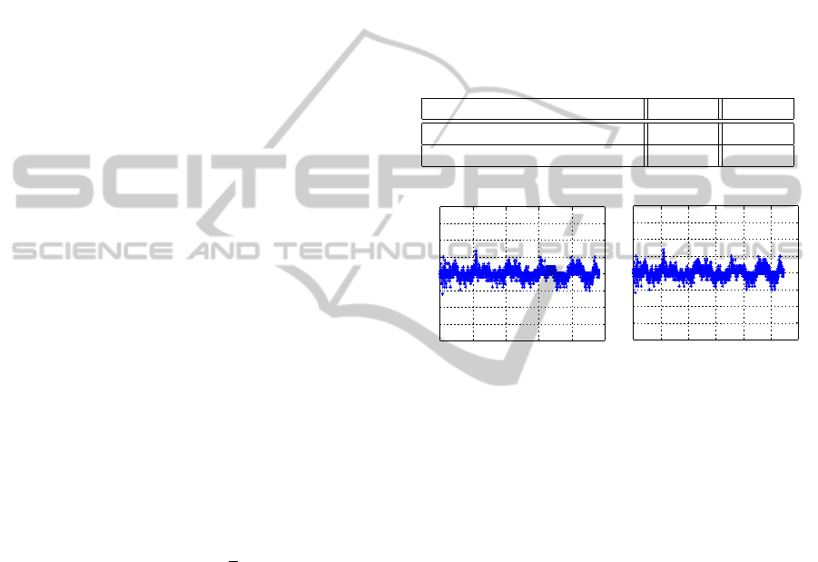
Table I shows the Root Mean Square for the predict-

ing and simulating errors. Better performances are

obtained using the polytopic bicycle model structure,

clearly because of introducing some a priori knowl-

edge of the dependence on the scheduling parameter

at the operating points.

Table 1: Root Mean Square.

Model SMB SFP

RMS(dgr/s) - predicted err. 0.0270 0.0277

RMS(dgr/s) - simulated err. 1.5851 3.4585

0 0.5 1 1.5 2 2.5 3

−2

−1.5

−1

−0.5

0.5

1.5

Erreur de prédiction - sfp

Temps(s)

Erreur de prédiction(degree/s)

0 0.5 1 1.5 2 2.5

−2

−1.5

−1

−0.5

0.5

1.5

Erreur de prédiction - smb

Temps(s)

Erreur de prédiction(degree/s)

Figure 4: Comparison between the real vehicle output and

the predicted outputs.

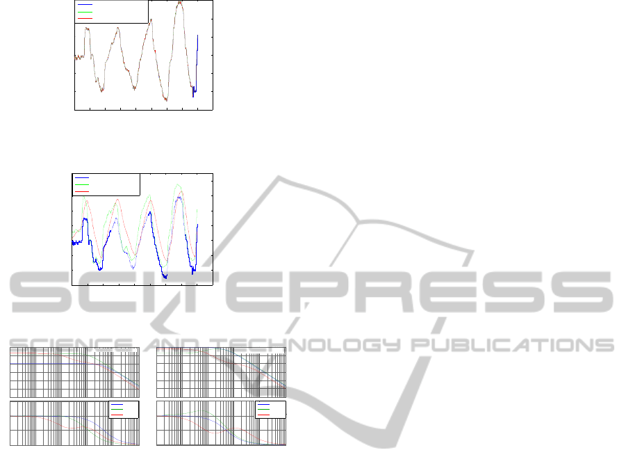
5.2 Validation

A new set of real data was used. We observe the re-

sults in time domain and analyze the model in the fre-

quency domain.

5.2.1 Time Domain Analysis

The predictor was simulated with the new data set. As

it can be seen in Figure 5 the outputs of the both struc-

tures reproduce well the system output. The nota-

tions Sfp correspond to the fully parameterized struc-

ture and Smb to bicycle model structure. In Figure 6,

the model was simulated with the new data set. As

we were looking for a predictor to minimize the pre-

diction error, it is normal that the error between the

predicted output of the model and the system output

being more important. We can observe better perfor-

mances in the case of the bicycle model structure, as

we have more a priori information about the system.

The validation also leads to insigniﬁcant prediction

error, for any vehicle velocity and reasonable simula-

tion error.

ICINCO2012-9thInternationalConferenceonInformaticsinControl,AutomationandRobotics

474

Time(s)

0 5 10 15 20 25 30 35 40 45

-6

-4

-2

(psi)/dt(degre

/sec)

Validation for predicted outputs

d(psi)/dt real

d(psi)/dt smb estimated

d(psi)/dt sfp estimated

Figure 5: Comparison between the real vehicle output and

the predicted output with a second set of data.

0 5 10 15 20 25 30 35 40 45

-6

-4

-2

Time(s)

d(psi)/dt(degr

e/sec)

Validation for simulated outputs

d(psi)/dt real

d(psi)/dt smb simulated

d(psi)/dt sfp simulated

Figure 6: Comparison between the real vehicle output and

the outputs simulated with a second set of data.

-40

-30

-20

-10

Magnitude (dB)

-2

-1

-90

-45

Phase (deg)

Frequency (rad/s)

sys anal

Smb

Sfp

Bode diagram for v = 100 Km/h

-40

-30

-20

-10

Magnitude (dB)

-2

-1

-90

-45

Phase (deg)

sys anal

Smb

Sfp

Frequency (rad/s)

Bode diagram for v= 60 Km/h

Figure 7: Bode diagrams for two arbitrary velocities.

5.2.2 Frequency Domain Analysis

Analysis of the analytical bicycle model, based on

the physical parameters given by the vehicle con-

structor, can be done for the chosen operating points.

The model is a second order with a zero that re-

duces the effect of the two poles, so it has the fre-

quency response similar to that of a 1

order system.

Bode diagrams (Figure 7) illustrate the inﬂuence of

the scheduling parameter on the characteristics of the

model, in the case of analytical model, high frequency

behavior is the same whatever the velocity is (as ex-

pected from the fact that C

is independent of the

velocity), modiﬁcations of the velocity induce mod-

iﬁcations of the static gain, and of the bandwidth in

accordance. The frequency response of the two struc-

tures was compared with the Bode diagram of the an-

alytical model, it can be observed that the identiﬁed

polytopic bicycle model structure tracks well the an-

alytical bicycle model dynamics at high frequencies,

because of the coherence of the form of the CB prod-

ucts of the two structures; which is not the case for

the fully parameterized polytopic model.

6 CONCLUSIONS

In this paper a LPV lateral behavior of a vehicle was

represented by a polytopic model. It was considered

that the system dependence on the scheduling param-

eter is known and a polytopic bicycle model struc-

ture was thus developed. The possibility of a model

whose parameter dependence is not known was also

taken into account, and a fully parameterized struc-

ture was created. Both models have been identiﬁed

from real data set recorded during an experiment with

a Laguna II vehicle. The pertinence of both identiﬁed

structures was carried out with a validation data set.

Better results were obtained with the polytopic bicy-

cle model structure, knowing that a priori information

of the system was available.

REFERENCES

Fujimori, A. and Ljung, L. (2005). Parameter estimation of

polytopic models for a linear parameter varying air-

craft system. submitted to Transactions of Japan So-

ciety for Aeronautical and Space Sciences (JSASS).

Heuberger, P. S. C. (2010). On the discretization of lpv

state-space representations. Transformation, 4(10):1–

29.

Ljung, L. (1999). System Identiﬁcation: Theory for the User

(2nd Edition). Prentice Hall.

Mammar, S. (2006). Memoire presente en vue d’obtenir

l’habilitation a diriger les recherches. Universite

d’Evry-Val d’Essone.

McKelvey, T. and Maureen, T. (1995). Identiﬁcation of

State-Space Models from Time and Frequency Data.

Osborne, M. R. (2007). Separable least squares, variable

projection, and the Gauss-Newton algorithm. Elec-

tronic Transactions on Numerical Analysis, 28:1–15.

Roweis, S. T. (1996). Levenberg-marquardt optimization.

IdentificationofPolytopicModelsforaLinearParameter-varyingSystemPerformedonaVehicle

475