Motion Detection and Velocity Estimation for Obstacle Avoidance using
3D Point Clouds
Sobers L. X. Francis, Sreenatha G. Anavatti and Matthew Garratt
SEIT, University of New South Wales@ADFA, Canberra, Australia
Keywords:
Scene Flow, Lucas/Kanade, Horn/Schunck, 3D ,PMD Camera, Motion Detection, Velocity Estimation.
Abstract:
This paper proposes a novel three dimensional (3D) velocity estimation method by using differential flow
techniques for the dynamic path planning of Autonomous Ground Vehicles (AGV) in a cluttered environment.
We provide a frame work for the computation of dense and non rigid 3D flow vectors from the range data,
obtained from the time-of-flight camera. Combined Lucas/Kanade and Horn/schunck approach is used to
estimate the velocity of the dynamic obstacles. The trajectory of the dynamic obstacle is predicted from
the direction of the 3D flow field and the estimated velocity. By experiments, the utility of the approach is
demonstrated with the results.
1 INTRODUCTION
Velocity estimation is an important research area in
autonomous mobile systems, which have been used in
dynamic path planning. The basic requirement for the
path planning is to plan the best possible path in such
a way that the AGV traverses the path and can replan
its path whenever it senses the obstacles in its way,
and can repeat the process until it reaches its goal.
In dynamic path planning, the vehicle has to modify
its path as per the dynamic characteristics of the sur-
roundings and plan to complete its ultimate task. In
dynamic environments, the obstacles will move ran-
domly causing the possibility of collision in the vehi-
cle’s path. In order to avoid the collision, the AGV
has to monitor the behaviour such as the position and
the orientation of the obstacles. So, it needs an opt
sensor that can sense the dynamic behaviour of the
obstacles.
Most of the researchers have been working on var-
ious image processing approaches in order to detect,
track and estimate the moving objects. The motion
estimation has been studied extensively over the past
two decades in the field of computer vision (B D Lu-
cas, 1981) (Horn and Schunck, 1981). Most of the
traditional methods are virtually based on analysing
the 2D data, ie images (Holte et al., 2010). These
2D images are only the projection of the actual 3D
data on the camera image plane. So the processing
of these images will depend upon the view point (not
on the actual information about the object). In order
to overcome this drawback the use of 3D information
has emerged.
The intensity based image processing techniques
are mainly based on grey scale or color in the im-
ages which is obtained from the conventional cam-
eras. The main disadvantages of these techniques are
that the image processing becomes inadequate in low
illumination conditions and when the objects and the
background look similar to each other (Yin, 2011).
As a result, three dimensional range data (x,y,z)
has been introduced. Usually there are three ba-
sic optical distance measurement principles (Ahlskog,
2007) such as Interferometry, Stereo/Triangulation
and Time-of-Flight [TOF] which can construct these
data (x,y, z). These range data can be used in flow
vector techniques to improve the quality of 3D object
segmentation, calculate object trajectories and time-
to-collision (Schmidt et al., 2008).
The objectiveof this paper is to detect the dynamic
obstacles and estimate the velocities in X,Y,Z direc-
tions based on the 3D point cloud from the Photonic
Mixer Device (PMD) camera. The paper uses the
combined Lucas/Kanade and Horn/Schunck differen-
tial flow techniques (Bauer et al., 2006), (Bruhn et al.,
2005) to estimate the velocities in 3D coordinates.
The paper is organised as follows: Section II de-
scribes about the PMD camera. Section III provides
the velocity estimation using the modified differential
flow technique. In Section IV, the experimental re-
sults are discussed. Section V summarises the work.
255
L. X. Francis S., G. Anavatti S. and Garratt M..
Motion Detection and Velocity Estimation for Obstacle Avoidance using 3D Point Clouds.
DOI: 10.5220/0004037502550259
In Proceedings of the 9th International Conference on Informatics in Control, Automation and Robotics (ICINCO-2012), pages 255-259
ISBN: 978-989-8565-22-8
Copyright
c
 2012 SCITEPRESS (Science and Technology Publications, Lda.)

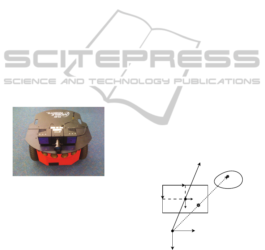
2 PMD CAMERA
We are using Photonic Mixer Device (PMD) camera,
a TOF camera in this work, in figure 1. A time of
flight camera is a system that works with the TOF
principles (Weingarten et al., 2004), and resembles a
LIDAR scanner. In the TOF unit (Lange, 2000), a
modulated light pulse is transmitted by the illumina-
tion source and the target distance is measured from
the time taken by the pulse to reflect from the target
and back to the receiving unit. PMD cameras can gen-
erate the range information, which is almost indepen-
dent of lighting conditions and visual appearance, and
a gray scale intensity image, similar to conventional
cameras. The coordinates of the obstacle with respect
to the PMD camera are obtained as a 200 by 200 ma-
trix, each element corresponding to a pixel. It pro-
vides fast acquisition of high resolution range data.
As the PMD range camera provides sufficient infor-
mation about the obstacles, it is proposed to estimate
the trajectory of the moving obstacles.
These TOF camera provide a 3D point cloud,
which is set of surface points in a three-dimensional
coordinate system (X,Y,Z), for all objects in the field
of view of the camera.
Figure 1: PMD Camera.
3 SCENE FLOW
Optical Flow (Barron et al., 1992)is an approximation
of the local image motion based upon local derivatives
in a given sequence of images. That is, in 2D it speci-
fies how much each image pixel moves between adja-
cent images while in 3D, it specifies how much each
volume voxel moves between adjacent volumes. The
moving patterns cause temporal varieties of the image
brightness. In general, the process of determining op-
tical flow is using a brightness constancy constraint
equation(BCCE). The spatiotemporal derivatives of
image intensity are used in differential techniques to
get the optical flow.
Differential techniques can be classified as local
and global. Local techniques involve the optimiza-
tion of a local energy, as in the Lucas and Kanade
method. The global techniques determine the flow
vector through minimization of a global energy, as in
Horn and Schunck. Local methods offer robustness
to noise, but lack the ability to produce dense optical
flow fields. Global techniques produce 100 percent
dense flow fields, but have a much larger sensitivity
to noise. The paper (Bauer et al., 2006) involves com-
bining local and global methods of Lucas-Kanade and
Horn-Schunck, to obtain a method which generates
dense optical flow under noisy image conditions.
Scene Flow (Vedula et al., 2005) is the three-
dimensional motion fields of points in the world; just
as optical flow is the 2D motion field of points in an
image. Any optical flow is simply the projection of
the scene flow onto the image plane of a camera. If
the world is completely non-rigid, the motions of the
points in the scene may all be independent of each
other. One representation of the scene motion is there-
fore a dense three-dimensional vector field defined for
every point on every surface in the scene.
These 2D images are only the projection of the
actual 3D data on the camera image plane, which
is illustrated in figure 2. Figure 2 shows a point
M=(X,Y,Z) from world coordinates which is pro-
jected and imaged on a point m = x,y in the camera’s
image plane. These coordinates are with respect to a
coordinate system whose origin is at the intersection
of the optical axis and the image plane, and whose x
and y axes are parallel to the X and Y axes (Iwadate,
2010). The three dimensional coordinates are based
on the optical projection centre C. Here, (u,v) are the
C
u
v
X
Y
Z
M = (X,Y,Z)
Object
m = (x,y)
x
y
Camera Coordinates
Image Coordinates
c
Figure 2: Camera Coordinates and Image coordinates.
camera pixel coordinates or image coordinates. The
point M on an object with coordinates (X,Y, Z) will be
imaged at some point m = (x,y) in the image plane.
In order to compute the 3D motion constraint equa-
tion (Barron and Thacker,2005), the derivativesof the
ICINCO2012-9thInternationalConferenceonInformaticsinControl,AutomationandRobotics
256

depth function with respect to the other world coordi-
nates have to be computed. For instance, the dynamic
object at (x,y,z) at time t is moved by (δx,δy, δz) to
(x + δx, y + δy, z + δz) over time δt. The 3D Mo-
tion Constraint Equation (1) is obtained after per-
forming 1
st
order Taylor series expansion (Barron and
Thacker, 2005).
R
x
V
x
+ R
y
V
y
+ R
z
V
z
+ R
t
= 0 (1)
where,
~
V = (V
x
,V
y
,V
z
) = (δx/δt,δy/δt,δz/δt) is the
3D volume velocity, ∇R = (R
x
,R
y
,R
z
) are the 3D spa-
tial derivatives and R
t
is the 3D temporal derivative.
It is the analogue of the brightness change constraint
equation (Spies et al., 2002) used in optical flow cal-
culation.
3.1 Lucas and Kanade
In practice, the Lucas/Kanade algorithm (B D Lu-
cas, 1981) is an intensity-based differential technique,
which assumes that the flow vector is constant within
a neighborhood region of pixels. The flow vectors
are calculated by applying a weighted least-squares
fit of local first-order constraints to a constant model
for
~
V in each spatial neighbourhood (Bauer et al.,
2006). The velocity estimate is given by minimizing
the equation as follows.
where W(x, y,z) denotes a Guassian Windowing func-
tion. The velocity estimates is given by (2).
~
V = [A
T
W
2
A]
−1
A
T
WB (2)
where,
A = [∇R(x
1
,y
1
,z
1
),...,∇R(x
n
,y
n
,z
n
)] (3)
W = diag[W(x
1
,y
1
,z
1
),...,W(x
n
,y
n
,z
n
)] (4)
B = −(R
t
(x
1
,y
1
,z
1
),...,R
t
(x
n
,y
n
,z
n
)) (5)
3.2 Horn and Schunck
Horn Schunck (Horn and Schunck, 1981) combines
the gradient constraints with a global smoothness
term. The flow velocity can be determined by min-
imizing the squared error quantity of constraint equa-
tion and smoothness constraint. The global smooth-
ness constraint is given by k∇V
x
k
2
,k∇V
y
k
2
,k∇V
z
k
2
and also expressed as (6).

∂V
x
∂x

2
+

∂V
x
∂y

2
+

∂V
x
∂x

2
+

∂V
y
∂x

2
+

∂V
y
∂y

2
+

∂V
y
∂z

2
+

∂V
z
∂x

2
+

∂V
z
∂y

2
+

∂V
z
∂z

2
,
(6)
The error to be minimised is defined in equation (7).
E
2
=
Z
D
(∇R.
~
V + R
t
)
2
+ α
2

k∇V
x
k
2
k∇V
y
k
2
k∇V
z
k
2

dxdydz (7)
where α is a weighting term that identifies the in-
fluence of smoothness constraint.
3.3 Combined Lucas/Kanade and
Horn/Schunck
The combined differential approach involves apply-
ing a locally implemented, weighted least squares fit
of local constraints to a constant model for flow ve-
locity, which is combined with the global smoothness
constraint. The velocity estimates can be minimised
by equation (8).
E
2
=
Z
D
(W
2
N
(∇R.
~
V + R
t
)
2
)
+ α
2

k∇V
x
k
2
k∇V
y
k
2
k∇V
z
k
2

dxdydz (8)
A
T
W
2
A is calculated as (9)
A
T
W
2
A =


∑
W
2
R
2
x
∑
W
2
R
x
R
y
∑
W
2
R
x
R
z
∑
W
2
R
x
R
y
∑
W
2
R
2
y
∑
W
2
R
y
R
z
∑
W
2
R
x
R
z
∑
W
2
R
y
R
z
∑
W
2
R
2
z


(9)
The velocity estimates can be solved through an iter-
ative process.
V
n+1
x
= V
n
x
−
W
2
N
R
x
(R
x
V
x
+ R
y
V
y
+ R
z
V
z
+ R
t
)
α
2
+W
2
N
(R
2
x
+ R
2
y
+ R
2
z
)
(10)
V
n+1
y
= V
n
y
−
W
2
N
R
y
(R
x
V
x
+ R
y
V
y
+ R
z
V
z
+ R
t
)
α
2
+W
2
N
(R
2
x
+ R
2
y
+ R
2
z
)
(11)
V
n+1
z
= V
n
z
−
W
2
N
R
z
(R
x
V
x
+ R
y
V
y
+ R
z
V
z
+ R
t
)
α
2
+W
2
N
(R
2
x
+ R
2
y
+ R
2
z
)
(12)
where, the average of previous velocity estimates (V
n
x
,
V
n
y
, V
n
z
) are used along with the derivates estimates to
obtain the new velocity estimates (V
n+1
x
, V
n+1
y
, V
n+1
z
).
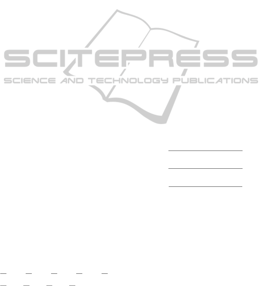
3.4 Experiment
The experiment is conducted by mounting the PMD
camera over the Pioneer 3DX mobile robot, AGV. In
our work, this PMD camera has been used as the vi-
sion sensor for efficient dynamic path planning. The
scenario has been developed such that a person is
walking towards the AGV from the far end. The task
is to detect and estimate the movement of the person.
So the relative distance between the vehicle and the
moving person is calculated using the camera. As the
MotionDetectionandVelocityEstimationforObstacleAvoidanceusing3DPointClouds
257

camera senses the three dimensional coordinates of
the person at different frame sequences, this 3D infor-
mation is utilised to estimate the resultant velocity by
using the combined Lucas/Kanade and Horn/Schunck
differential techniques.
Two frames of 3D point clouds (R
1
(x,y,z,t),
R
2
(x,y,z,t)) are stored, as shown in figure 3 and 4.
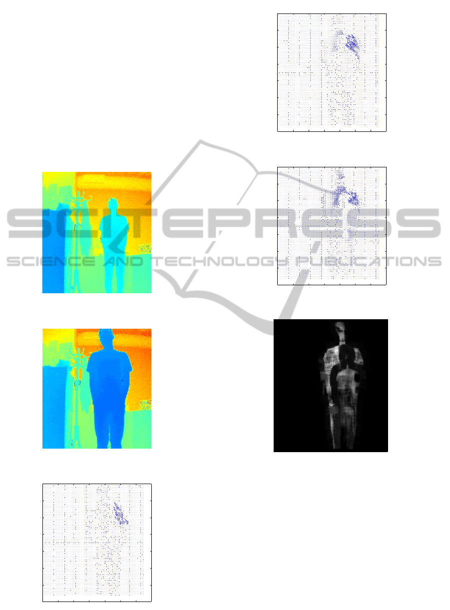
Figure 5, figure 6 and figure 7 show the velocity vec-
tors along X,Y,Z direction. The resultant of these
three vectors (V
x
,V
y
,V
z
) are shown in 3D scale, fig-
ure 9. The vector flow which is also generated using
the range data, r(x,y,t),with r being the distance and
x,y being camera pixel coordinates, is shown in figure
10.
Figure 3: Frame 1.
Figure 4: Frame 2.
Figure 5: Flow vector along X direction.
Figure 6: Flow vector along Y direction.
Figure 7: Flow vector along Z direction.
Figure 8: Edge Detection.
4 CONCLUSIONS
The paper shows the novel approach for veloc-
ity estimation using combined Lucas/Kanade and
Horn/Schunck range-based differential technique. As
the PMD camera gives suffient information about the
obstacles, it is integrated with a Pioneer mobile robot
to develop an efficient dynamic path planning in a
cluttered environment. Our future work will focus on
prediction of the dynamic obstacle’s trajectory using
the estimated velocity.
ICINCO2012-9thInternationalConferenceonInformaticsinControl,AutomationandRobotics
258

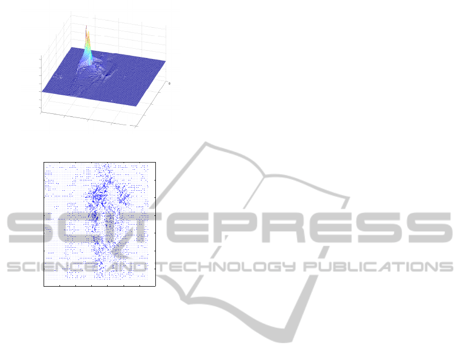
Figure 9: Resultant Vectors in 3D Scale.
Figure 10: Flow Vectors using PMD Range data.
REFERENCES
Ahlskog, M. (2007). 3D Vision. Master’s thesis, Depart-
ment of Computer Science and Electronics, Mlardalen
University.
B D Lucas, T. K. (1981). An iterative image restoration
technique with an application to stereo vision. In
5th International Joint Conference on Artificial Intel-
ligence, pages 674–679.
Barron, J., Fleet, D., Beauchemin, S., and Burkitt, T.
(1992). Performance of optical flow techniques. In
Computer Vision and Pattern Recognition, 1992. Pro-
ceedings CVPR ’92., 1992 IEEE Computer Society
Conference on, pages 236 –242.
Barron, J. L. and Thacker, N. A. (2005). Tutorial: comput-
ing 2D and 3D optical flow. In Tina Memo, number
2004-012.
Bauer, N., Pathirana, P., and Hodgson, P. (2006). Robust
Optical Flow with Combined Lucas-Kanade/Horn-
Schunck and Automatic Neighborhood Selection. In
Information and Automation, 2006. ICIA 2006. Inter-
national Conference on, pages 378 –383.
Bruhn, A., Weickert, J., and Schn¨orr, C. (2005). Lu-
cas/Kanade meets Horn/Schunck: combining local
and global optic flow methods. Int. J. Comput. Vision,
61(3):211–231.
Holte, M., Moeslund, T., and Fihl, P. (2010). View-invariant
gesture recognition using 3D optical flow and har-
monic motion context. Computer Vision and Image
Understanding, 114(12):1353 – 1361.
Horn, B. K. P. and Schunck, B. G. (1981). Determining
optical flow. Artifical Intelligence, 17:185–203.
Iwadate, Y. (2010). Outline of three-dimensional image pro-
cessing.
Lange, R. (2000). 3D time-of-flight distance measurement
with custom solid-state image sensors in CMOS/CCD-
technology. PhD thesis, Dep. of Electrical Engineer-
ing and Computer Science, University of Siegen.
Schmidt, M., Jehle, M., and Jahne, B. (2008). Range flow
estimation based on photonic mixing device data. Int.
J. Intell. Syst. Technol. Appl., 5(3/4):380–392.
Spies, H., Jahne, B., and Barron, J. (2002). Range flow es-
timation. Computer Vision and Image Understanding,
85(3):209–231.
Vedula, S., Rander, P., Collins, R., and Kanade, T.
(2005). Three-dimensional scene flow. Pattern Anal-
ysis and Machine Intelligence, IEEE Transactions on,
27(3):475 –480.
Weingarten, J. W., Gruener, G., and Siegwart, R. (2004).
A state-of-the-art 3D sensor for robot navigation. In
Intelligent Robots and Systems. In In IEEE/RSJ Int.
Conf. on Intelligent Robots and Systems, volume 3,
pages 2155–2160.
Yin, Xiang; Noguchi, N. (2011). Motion detection and
tracking using the 3d-camera. In 18th IFAC World
Congress, volume 18, pages 14139–14144.
MotionDetectionandVelocityEstimationforObstacleAvoidanceusing3DPointClouds
259